# Load needed libraries
library(sf)Vector Data
Library Loading
Before we can dive into “actual” spatial work we’ll need to load some libraries.
Load sf to work with vector data.
Load the geopandas library to work with vector data. We’ll also load the os library to deal with file path issues.
# Load needed libraries
import os
import geopandas as gpd
Loading Vector Data
To demonstrate vector data operations we’ll use data on the counties in North Carolina (USA). Note that some minor preparatory work was necessary to get the data ready for our purposes here and is preserved in this folder of the website’s GitHub repository.
There are several R packages for working with vector data but we’ll focus on sf.
# Load a shapefile of county borders
vect_r <- sf::st_read(dsn = file.path("data", "nc.shp"))
Reading layer `nc' from data source
`/Users/nick.lyon/Documents/coding/collab_r-python-bilingualism/data/nc.shp'
using driver `ESRI Shapefile'
Simple feature collection with 100 features and 14 fields
Geometry type: MULTIPOLYGON
Dimension: XY
Bounding box: xmin: -84.32377 ymin: 33.88212 xmax: -75.45662 ymax: 36.58973
Geodetic CRS: WGS 84# Check the class of this object
class(vect_r)[1] "sf" "data.frame"The geopandas library will be our focal library for vector operations with Python.
# Load a shapefile of county borders
vect_py = gpd.read_file(os.path.join("data", "nc.shp"))

# Check the class of this object
type(vect_py)
<class 'geopandas.geodataframe.GeoDataFrame'>Vector Data Structure
Note that vector data are often structurally similar to tabular data so some of the operations you can use in Pandas/Tidyverse variables/objects can be performed on these data. To demonstrate this, lets check the columns included in this vector data.
In R we can explore vector data using the str function. Note that the spatial information is stored in the “geometry” column; see the strange class attribute?
# Check columns
str(vect_r)
Classes 'sf' and 'data.frame': 100 obs. of 15 variables:
$ AREA : num 0.114 0.061 0.143 0.07 0.153 0.097 0.062 0.091 0.118 0.124 ...
$ PERIMETER: num 1.44 1.23 1.63 2.97 2.21 ...
$ CNTY_ : num 1825 1827 1828 1831 1832 ...
$ CNTY_ID : num 1825 1827 1828 1831 1832 ...
$ NAME : chr "Ashe" "Alleghany" "Surry" "Currituck" ...
$ FIPS : chr "37009" "37005" "37171" "37053" ...
$ FIPSNO : num 37009 37005 37171 37053 37131 ...
$ CRESS_ID : int 5 3 86 27 66 46 15 37 93 85 ...
$ BIR74 : num 1091 487 3188 508 1421 ...
$ SID74 : num 1 0 5 1 9 7 0 0 4 1 ...
$ NWBIR74 : num 10 10 208 123 1066 ...
$ BIR79 : num 1364 542 3616 830 1606 ...
$ SID79 : num 0 3 6 2 3 5 2 2 2 5 ...
$ NWBIR79 : num 19 12 260 145 1197 ...
$ geometry :sfc_MULTIPOLYGON of length 100; first list element: List of 1
..$ :List of 1
.. ..$ : num [1:27, 1:2] -81.5 -81.5 -81.6 -81.6 -81.7 ...
..- attr(*, "class")= chr [1:3] "XY" "MULTIPOLYGON" "sfg"
- attr(*, "sf_column")= chr "geometry"
- attr(*, "agr")= Factor w/ 3 levels "constant","aggregate",..: NA NA NA NA NA NA NA NA NA NA ...
..- attr(*, "names")= chr [1:14] "AREA" "PERIMETER" "CNTY_" "CNTY_ID" ...In Python we can explore vector data via the dtypes attribute (which is also found in ‘normal’ tabular data variables). Note that the spatial information is stored in the “geometry” column; see the strange type attribute?
# Check columns
vect_py.dtypes
AREA float64
PERIMETER float64
CNTY_ float64
CNTY_ID float64
NAME object
FIPS object
FIPSNO float64
CRESS_ID int32
BIR74 float64
SID74 float64
NWBIR74 float64
BIR79 float64
SID79 float64
NWBIR79 float64
geometry geometry
dtype: objectChecking Vector CRS
As noted earlier, the very first thing we should do after reading in spatial data is check the coordinate reference system!
We can check the CRS with the st_crs function (from sf).
# Check the CRS of the shapefile
sf::st_crs(x = vect_r)
Coordinate Reference System:
User input: WGS 84
wkt:
GEOGCRS["WGS 84",
DATUM["World Geodetic System 1984",
ELLIPSOID["WGS 84",6378137,298.257223563,
LENGTHUNIT["metre",1]]],
PRIMEM["Greenwich",0,
ANGLEUNIT["degree",0.0174532925199433]],
CS[ellipsoidal,2],
AXIS["latitude",north,
ORDER[1],
ANGLEUNIT["degree",0.0174532925199433]],
AXIS["longitude",east,
ORDER[2],
ANGLEUNIT["degree",0.0174532925199433]],
ID["EPSG",4326]]Python stores vector CRS as an attribute.
# Check the CRS of the shapefile
vect_py.crs
<Geographic 2D CRS: EPSG:4326>
Name: WGS 84
Axis Info [ellipsoidal]:
- Lat[north]: Geodetic latitude (degree)
- Lon[east]: Geodetic longitude (degree)
Area of Use:
- name: World.
- bounds: (-180.0, -90.0, 180.0, 90.0)
Datum: World Geodetic System 1984 ensemble
- Ellipsoid: WGS 84
- Prime Meridian: GreenwichTransforming Vector CRS
Once we know the current CRS, we can transform into a different coordinate reference system as needed. Let’s transform from WGS84 into another commonly-used CRS: Albers Equal Area (EPSG code 3083).
Note that while transforming a raster’s CRS is very computationally intensive, transforming vector data CRS is much faster. If you are trying to use vector and raster data together but they don’t use the same CRS it can be quicker to transform the vector data to match the raster data (rather than vice versa).
For CRS transformations in R we can use the st_transform function.
# Transform the shapefile CRS
vect_alber_r <- sf::st_transform(x = vect_r, crs = 3083)

# Re-check the CRS to confirm it worked
sf::st_crs(vect_alber_r)
Coordinate Reference System:
User input: EPSG:3083
wkt:
PROJCRS["NAD83 / Texas Centric Albers Equal Area",
BASEGEOGCRS["NAD83",
DATUM["North American Datum 1983",
ELLIPSOID["GRS 1980",6378137,298.257222101,
LENGTHUNIT["metre",1]]],
PRIMEM["Greenwich",0,
ANGLEUNIT["degree",0.0174532925199433]],
ID["EPSG",4269]],
CONVERSION["Texas Centric Albers Equal Area",
METHOD["Albers Equal Area",
ID["EPSG",9822]],
PARAMETER["Latitude of false origin",18,
ANGLEUNIT["degree",0.0174532925199433],
ID["EPSG",8821]],
PARAMETER["Longitude of false origin",-100,
ANGLEUNIT["degree",0.0174532925199433],
ID["EPSG",8822]],
PARAMETER["Latitude of 1st standard parallel",27.5,
ANGLEUNIT["degree",0.0174532925199433],
ID["EPSG",8823]],
PARAMETER["Latitude of 2nd standard parallel",35,
ANGLEUNIT["degree",0.0174532925199433],
ID["EPSG",8824]],
PARAMETER["Easting at false origin",1500000,
LENGTHUNIT["metre",1],
ID["EPSG",8826]],
PARAMETER["Northing at false origin",6000000,
LENGTHUNIT["metre",1],
ID["EPSG",8827]]],
CS[Cartesian,2],
AXIS["easting (X)",east,
ORDER[1],
LENGTHUNIT["metre",1]],
AXIS["northing (Y)",north,
ORDER[2],
LENGTHUNIT["metre",1]],
USAGE[
SCOPE["State-wide spatial data presentation requiring true area measurements."],
AREA["United States (USA) - Texas."],
BBOX[25.83,-106.66,36.5,-93.5]],
ID["EPSG",3083]] Python CRS re-projections use the same process but the relevant method is to_crs.
# Transform the shapefile CRS
vect_alber_py = vect_py.to_crs("EPSG:3083")

# Re-check the CRS to confirm it worked
vect_alber_py.crs
<Projected CRS: EPSG:3083>
Name: NAD83 / Texas Centric Albers Equal Area
Axis Info [cartesian]:
- X[east]: Easting (metre)
- Y[north]: Northing (metre)
Area of Use:
- name: United States (USA) - Texas.
- bounds: (-106.66, 25.83, -93.5, 36.5)
Coordinate Operation:
- name: Texas Centric Albers Equal Area
- method: Albers Equal Area
Datum: North American Datum 1983
- Ellipsoid: GRS 1980
- Prime Meridian: GreenwichMap Making with Vector Data
Once you’ve checked the CRS and confirmed it is appropriate, you may want to make a simple map. Again, because these data variables/objects have a similar structure to ‘normal’ tabular data we can use many of the same tools without modification.
The base R function plot works for spatial data too! Though note that it will make a separate map panel for each column in the data so we’ll need to pick a particular column to get just one map.
# Make a map
plot(vect_r["AREA"])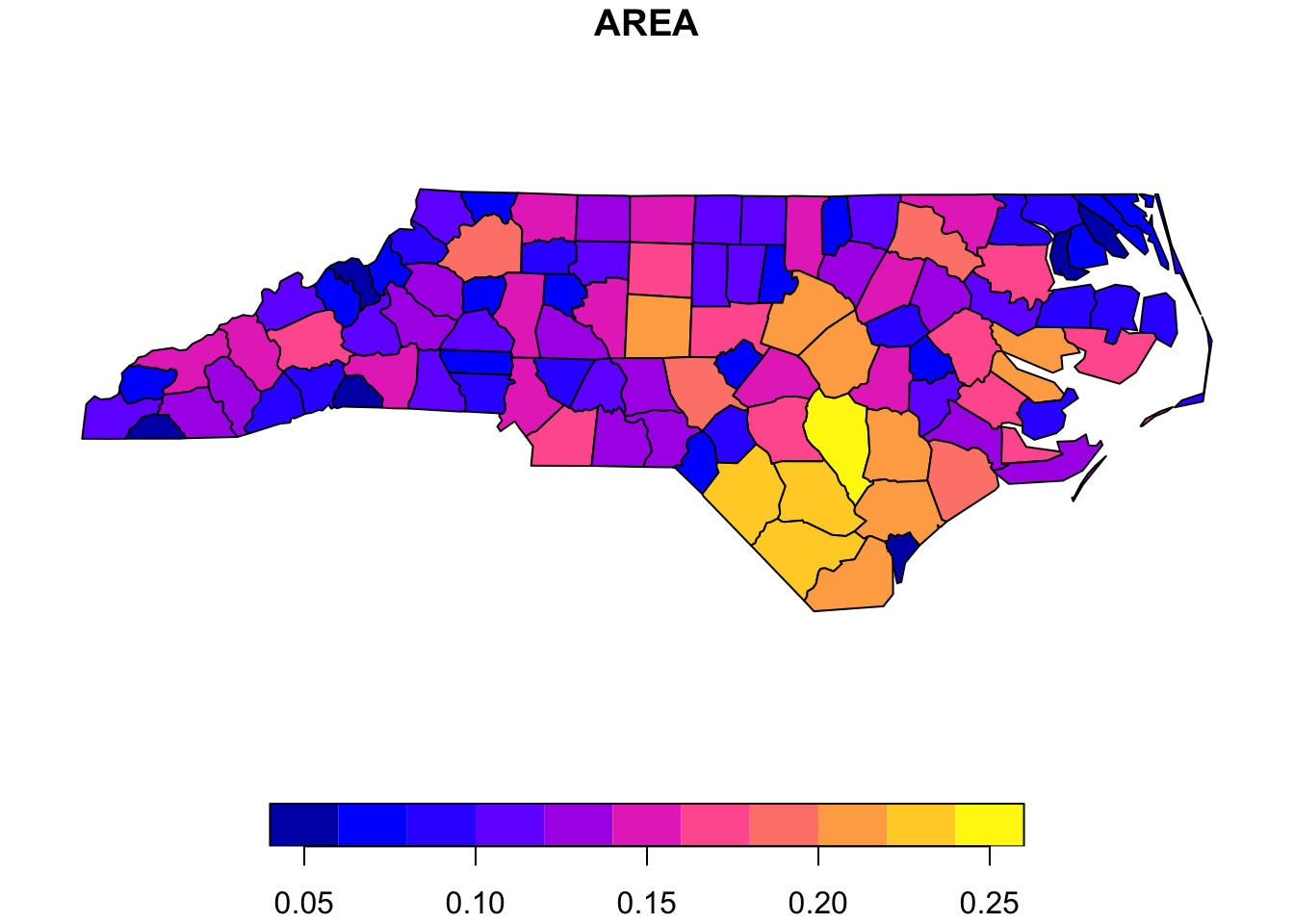
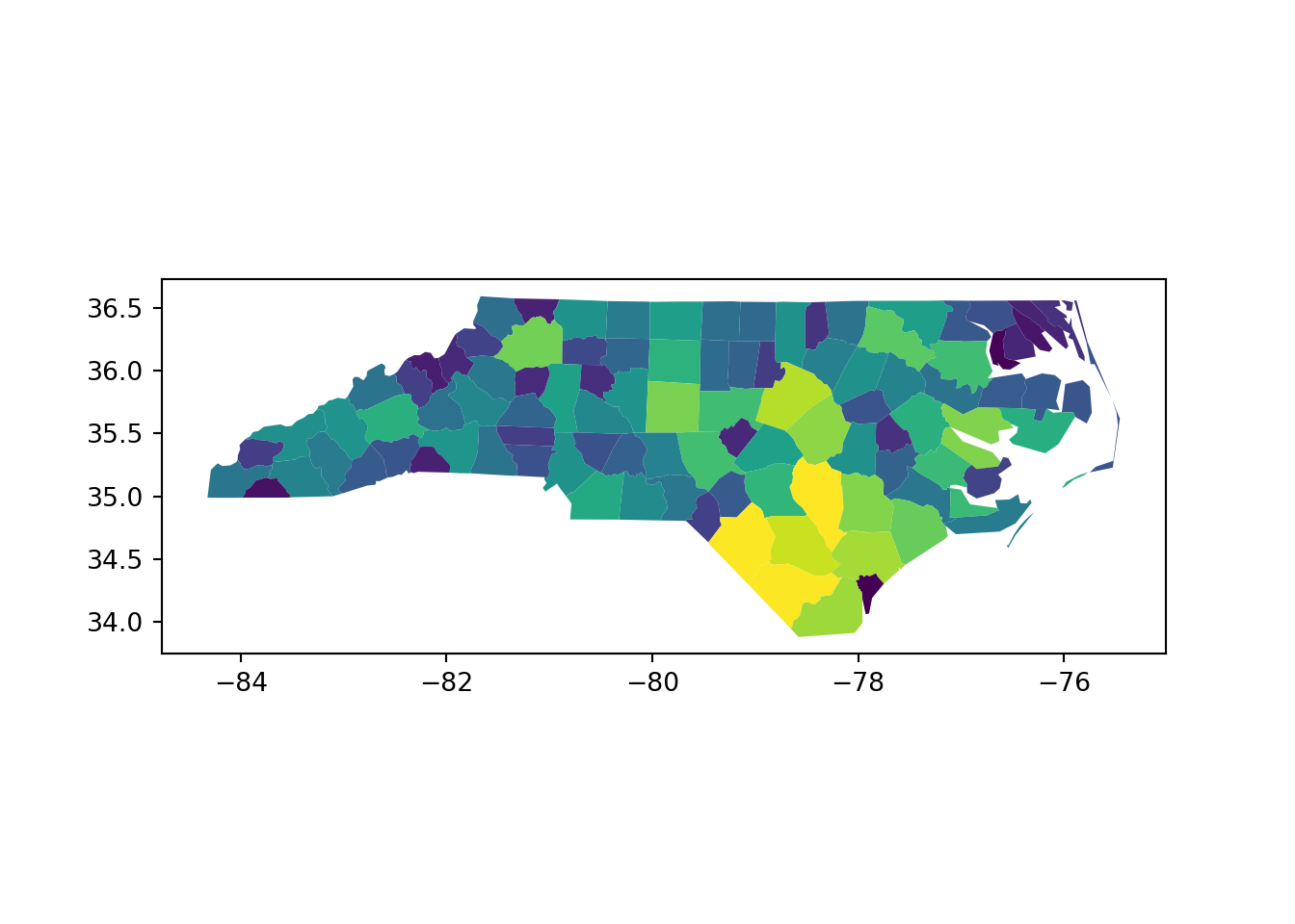
Python uses the plot method for this type of variable. Though note that without specifying the “column” argument we will get the map but every polygon will be filled with the default grey-blue color rather than informatively tied to another column in the data.
# Make a map
vect_py.plot(column = "AREA")