Spatial Fundamentals

Spatial Data Types

There are two primary types of spatial data: raster and vector data. Python and R can both handle either of these types so coding language doesn’t matter but there are fundamental structural differences between the two data types. See below for more information about each.

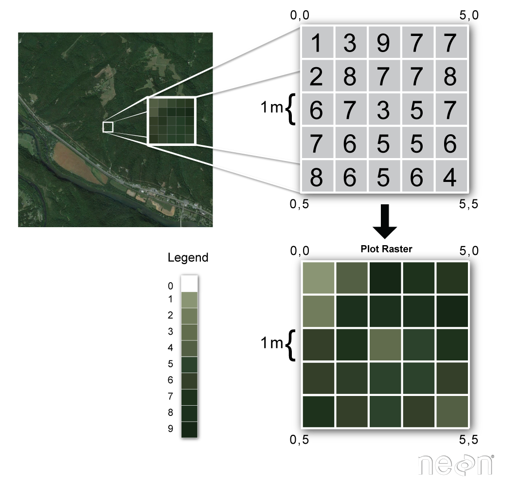
Raster data stores information in pixels. Each pixel is located at a specific geographic location (i.e., a specific X and Y coordinate pair). These pixel values can be continuous (e.g., rainfall, elevation, etc.) or categorical (e.g., land cover categories, date of first green up, etc.). Even if you’ve never worked with spatial data before you’ve certainly worked with rasters: technically every digital image is a raster!

Raster files are typically GeoTIFFs and use the .tif extension.

Consider this visual depiction of raster data:

Picture of a forest with an inset showing how the pixels in that image relate to information stored in each pixel
Image Source - National Ecological Observatory Network (NEON)

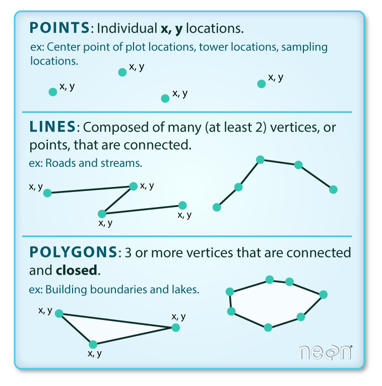
Vector data store information in “features”. These features use specific geographic points (again, think X and Y coordinates) and store information about the geometric relationship among features. This allows vector data to be in terms of particular geometries like points, lines, or polygons.

Vector data are typically preserved as shapefiles and use several extensions. When we refer to shapefiles in code we only refer to the .shp file but there are several associated files that must also be present in the same folder for the data to be read properly. These usually include .dbf, .prj, and .shx but there may sometimes also be a .xml file or two. For our purposes, the specifics of these files are not relevant but it is important to remember that you will need them in order to work with vector data.

Consider this visual depiction of vector data:

Diagram of points, lines (points connected by lines), and polygons (three or more points that define the edges of a shape)
Image Source - National Ecological Observatory Network (NEON)

Library Loading

Before we can dive into “actual” spatial work we’ll need to load some libraries.

Load terra and sf to work with raster and vector data respectively.

# Load needed libraries
library(terra)
library(sf)

Load the rioxarray, rasterio, and geopandas libraries to work with raster and vector data. We’ll also load the os library to deal with file path issues.

# Load needed libraries
import rasterio as rio
import rioxarray as rxr
import geopandas as gpd
import os

Coordinate Reference Systems (CRS)

While raster and vector data may both refer to non-spatial or spatial data, true spatial data requires a coordinate reference system (CRS). CRS has a very specific format that all geospatial applications (including Python and R!) use to display/process the data correctly. CRS includes three components:

  1. Datum – a model for the shape of the earth. It defines the starting coordinate pair and angular units that–when used with the starting point–define a particular spot on the planet. There can be global datums (e.g., WGS84, NAD83, etc.) that apply anywhere on the planet and local datums that work well for a particular area but do not work outside of that area
  2. Projection – mathematical transformation to get from a round planet to a flat map
  3. Additional Parameters – any other information necessary to support the projection (e.g., the coordinates of the center of the map, etc.)

A hopefully useful analogy is to consider the datum as a choice between a set of citrus fruits of varying shapes (e.g., lemon, orange, grapefruit, etc.) while the projection is a set of instructions on how to flatten the peel of the chosen fruit.

CRS Importance

Coordinate reference systems may sound dry and uninteresting–even in a pretty technical coding context–but they are vitally important! For many scientific purposes we want to know how a set of points intersect with a given map or how well several maps line up. To answer questions like these or interpret virtually any geospatial information, we must make sure that each spatial component uses the same CRS. Some coordinate reference systems use similar units which can mean a quick glance makes all spatial data seem interoperable while in reality the data cannot be directly compared without transforming to a standard CRS.

A rule of thumb that may help is that every spatial script you write should be very careful to check the CRS(s) used by the data.

Working with Rasters

To demonstrate raster data operations we’ll use NASA’s Shuttle Radar Topography Mission Global 3 arc second elevation data. Note that some minor preparatory work was necessary to get the data ready for our purposes here and is preserved in this folder of the website’s GitHub repository.

Loading Rasters

We can begin by reading in the data.

There are several R packages for working with raster data but we’ll focus on terra.

# Load a raster of elevation data
rast_r <- terra::rast(x = file.path("data", "elevation.tif"))

# Check the class of this object
class(rast_r)
[1] "SpatRaster"
attr(,"package")
[1] "terra"

The rioxarray library will be our focal library for raster operations with [ Python].

pd.read_csv(os.path.join(“data”, “verts.csv”))

# Load a raster of elevation data
rast_py = rxr.open_rasterio(os.path.join("data", "elevation.tif"), masked = True).squeeze()

# Check the type of this variable
type(rast_py.rio.crs)
<class 'rasterio.crs.CRS'>

Checking Raster CRS

As noted earlier, the very first thing we should do after reading in spatial data is check the coordinate reference system!

We can check the CRS with the crs function (from terra).

# Check the CRS of the elevation data
terra::crs(x = rast_r)
[1] "GEOGCRS[\"WGS 84\",\n    ENSEMBLE[\"World Geodetic System 1984 ensemble\",\n        MEMBER[\"World Geodetic System 1984 (Transit)\"],\n        MEMBER[\"World Geodetic System 1984 (G730)\"],\n        MEMBER[\"World Geodetic System 1984 (G873)\"],\n        MEMBER[\"World Geodetic System 1984 (G1150)\"],\n        MEMBER[\"World Geodetic System 1984 (G1674)\"],\n        MEMBER[\"World Geodetic System 1984 (G1762)\"],\n        MEMBER[\"World Geodetic System 1984 (G2139)\"],\n        ELLIPSOID[\"WGS 84\",6378137,298.257223563,\n            LENGTHUNIT[\"metre\",1]],\n        ENSEMBLEACCURACY[2.0]],\n    PRIMEM[\"Greenwich\",0,\n        ANGLEUNIT[\"degree\",0.0174532925199433]],\n    CS[ellipsoidal,2],\n        AXIS[\"geodetic latitude (Lat)\",north,\n            ORDER[1],\n            ANGLEUNIT[\"degree\",0.0174532925199433]],\n        AXIS[\"geodetic longitude (Lon)\",east,\n            ORDER[2],\n            ANGLEUNIT[\"degree\",0.0174532925199433]],\n    USAGE[\n        SCOPE[\"Horizontal component of 3D system.\"],\n        AREA[\"World.\"],\n        BBOX[-90,-180,90,180]],\n    ID[\"EPSG\",4326]]"

Python stores raster CRS as an attribute.

# Check the CRS of the elevation data
rast_py.rio.crs
CRS.from_epsg(4326)

You may note in the above operations that Python and R seem to be returning different information for the same data. In fact they are saying the same thing just in slightly different ways. R is telling us the name of the coordinate reference system (World Geodetic System 1984) while Python is giving us the four-digit “EPSG” code. For context, the European Petroleum Survey Group (EPSG) is a major authority on accepted coordinate reference systems. Each CRS is given a unique, four-digit code. As you may now be able to guess, “4326” is the EPSG code for the World Geodetic System 1984 CRS!

This CRS (WGS84) is an especially common one so you may eventually commit its EPSG code to memory but often you’ll encounter either CRS names or EPSG codes with which you are not familiar. It may not sound like sage advice but it can be simplest to just use whichever piece of information your coding language returns to Google the “missing” information.

Transforming Raster CRS

Once we know the current CRS, we can transform into a different coordinate reference system as needed. Let’s transform from WGS84 into another commonly-used CRS: Albers Equal Area (EPSG code 3083).

Quick warning, transforming rasters can take a long time and is very computationally intensive. It’ll work for a relatively small raster like the one we’re working with here but in general you should be careful with attempting to re-project a raster into a different CRS.

For CRS transformations in R we can use the project function (pronounced like the verb not the noun).

# Transform the raster CRS
rast_alber_r <- terra::project(x = rast_r, y = "epsg:3083")

# Re-check the CRS to confirm it worked
terra::crs(rast_alber_r)
[1] "PROJCRS[\"NAD83 / Texas Centric Albers Equal Area\",\n    BASEGEOGCRS[\"NAD83\",\n        DATUM[\"North American Datum 1983\",\n            ELLIPSOID[\"GRS 1980\",6378137,298.257222101,\n                LENGTHUNIT[\"metre\",1]]],\n        PRIMEM[\"Greenwich\",0,\n            ANGLEUNIT[\"degree\",0.0174532925199433]],\n        ID[\"EPSG\",4269]],\n    CONVERSION[\"Texas Centric Albers Equal Area\",\n        METHOD[\"Albers Equal Area\",\n            ID[\"EPSG\",9822]],\n        PARAMETER[\"Latitude of false origin\",18,\n            ANGLEUNIT[\"degree\",0.0174532925199433],\n            ID[\"EPSG\",8821]],\n        PARAMETER[\"Longitude of false origin\",-100,\n            ANGLEUNIT[\"degree\",0.0174532925199433],\n            ID[\"EPSG\",8822]],\n        PARAMETER[\"Latitude of 1st standard parallel\",27.5,\n            ANGLEUNIT[\"degree\",0.0174532925199433],\n            ID[\"EPSG\",8823]],\n        PARAMETER[\"Latitude of 2nd standard parallel\",35,\n            ANGLEUNIT[\"degree\",0.0174532925199433],\n            ID[\"EPSG\",8824]],\n        PARAMETER[\"Easting at false origin\",1500000,\n            LENGTHUNIT[\"metre\",1],\n            ID[\"EPSG\",8826]],\n        PARAMETER[\"Northing at false origin\",6000000,\n            LENGTHUNIT[\"metre\",1],\n            ID[\"EPSG\",8827]]],\n    CS[Cartesian,2],\n        AXIS[\"easting (X)\",east,\n            ORDER[1],\n            LENGTHUNIT[\"metre\",1]],\n        AXIS[\"northing (Y)\",north,\n            ORDER[2],\n            LENGTHUNIT[\"metre\",1]],\n    USAGE[\n        SCOPE[\"State-wide spatial data presentation requiring true area measurements.\"],\n        AREA[\"United States (USA) - Texas.\"],\n        BBOX[25.83,-106.66,36.5,-93.5]],\n    ID[\"EPSG\",3083]]"

Python CRS re-projections have slightly more steps to work through.

# Create a CRS variable for the desired ending CRS
wgs84_crs = rio.crs.CRS.from_string("EPSG:3083")

# Reproject the raster we had
rast_alber_py = rast_py.rio.reproject(wgs84_crs)

# Re-check the CRS to confirm it worked
rast_alber_py.rio.crs
CRS.from_epsg(3083)

Working with Vector Data

Loading Vector Data

Checking Vector CRS

Transforming Vector CRS

Additional Resources

Spatial operations have gotten a ton of attention in both Python and R! This website is mostly focused on translating between the two languages though so much of this nuance is not covered here. For those interested in a deeper dive in spatial computing, consider the following.