Overview
The supportR package is an amalgam of distinct functions
I’ve written to accomplish small data wrangling, quality control, or
visualization tasks. These functions tend to be short and
narrowly-defined. An additional consequence of the motivation for
creating them is that they tend to not be inter-related or united by a
common theme. If this vignette feels somewhat scattered because of that,
I hope it doesn’t negatively affect how informative it is or your
willingness to adopt supportR into your scripts!
This vignette describes the main functions of supportR
using the examples included in each function.
Data Wrangling
In order to demonstrate some of the data wrangling functions of
supportR, we’ll use some some example data from Dr. Allison Horst’s palmerpenguins
R package.
# Check the structure of the penguins dataset
str(penguins)
#> 'data.frame':    344 obs. of  8 variables:
#>  $ species          : Factor w/ 3 levels "Adelie","Chinstrap",..: 1 1 1 1 1 1 1 1 1 1 ...
#>  $ island           : Factor w/ 3 levels "Biscoe","Dream",..: 3 3 3 3 3 3 3 3 3 3 ...
#>  $ bill_length_mm   : num  39.1 39.5 40.3 NA 36.7 39.3 38.9 39.2 34.1 42 ...
#>  $ bill_depth_mm    : num  18.7 17.4 18 NA 19.3 20.6 17.8 19.6 18.1 20.2 ...
#>  $ flipper_length_mm: int  181 186 195 NA 193 190 181 195 193 190 ...
#>  $ body_mass_g      : int  3750 3800 3250 NA 3450 3650 3625 4675 3475 4250 ...
#>  $ sex              : Factor w/ 2 levels "female","male": 2 1 1 NA 1 2 1 2 NA NA ...
#>  $ year             : int  2007 2007 2007 2007 2007 2007 2007 2007 2007 2007 ...
With that data loaded, we can use the summary_table
function to quickly get group-wise summaries and retrieve generally
useful summary statistics.
The groups argument supports a vector of all of the
column names to group by while response must be a single
numeric column. The drop_na argument allows group
combinations that result in an NA to be automatically dropped (i.e., if
a penguin didn’t have an island listed that would be dropped). The mean,
standard deviation (SD), sample size, and standard error (SE) are all
returned to facilitate easy figure creation. There is also a
round_digits argument that lets you specify how many digits
you’d like to retain for the mean, SD, and SE.
# Summarize the data
supportR::summary_table(data = penguins, groups = c("species", "island"),
                        response = "bill_length_mm", drop_na = TRUE)
#>     species    island  mean std_dev sample_size std_error
#> 1    Adelie    Biscoe 38.98    2.48          44      0.37
#> 2    Adelie     Dream 38.50    2.47          56      0.33
#> 3    Adelie Torgersen 38.95    3.03          52      0.42
#> 4 Chinstrap     Dream 48.83    3.34          68      0.41
#> 5    Gentoo    Biscoe 47.50    3.08         124      0.28
The safe_rename function allows–perhaps
predictably–“safe” renaming of column names in a given data object. The
‘bad’ column names and corresponding ‘good’ names must be specified. The
order of entries in the two vectors must match (i.e., the first bad name
will be replaced with the first good name), but that order need not
match the order in which they occur in the data!
# Make a dataframe to demonstrate
df <- data.frame("first" = 1:3, "middle" = 4:6, "second" = 7:9)

# Invoke the function
safe_rename(data = df, bad_names = c("second", "middle"),
            good_names = c("third", "second"))
#>   first second third
#> 1     1      4     7
#> 2     2      5     8
#> 3     3      6     9
crop_tri allows dropping one “triangle” of a symmetric
dataframe / matrix. It also includes a drop_diag argument
that accepts a logical for whether to drop the diagonal of the data
object. This is primarily useful (I find) in allowing piping through
this function as opposed to using the base R notation for removing a
triangle of a symmetric data object.
# Define a simple matrix wtih symmetric dimensions
mat <- matrix(data = c(1:2, 2:1), nrow = 2, ncol = 2)

# Crop off it's lower triangle
supportR::crop_tri(data = mat, drop_tri = "lower", drop_diag = FALSE)
#>      [,1] [,2]
#> [1,]    1    2
#> [2,]   NA    1

# Drop the diagonal as well
supportR::crop_tri(data = mat, drop_tri = "lower", drop_diag = TRUE)
#>      [,1] [,2]
#> [1,]   NA    2
#> [2,]   NA   NA
array_melt allows users to ‘melt’ an array of dimensions
X, Y, and Z into a dataframe containing columns “x”, “y”, “z”, and
“value” where “value” is whatever was stored at those coordinates in the
array.
# Make data to fill the array
vec1 <- c(5, 9, 3)
vec2 <- c(10:15)

# Create dimension names (x = col, y = row, z = which matrix)
x_vals <- c("Col_1","Col_2","Col_3")
y_vals <- c("Row_1","Row_2","Row_3")
z_vals <- c("Mat_1","Mat_2")

# Make an array from these components
g <- array(data = c(vec1, vec2), dim = c(3, 3, 2),
           dimnames = list(x_vals, y_vals, z_vals))

# "Melt" the array into a dataframe
melted <- supportR::array_melt(array = g)

# Look at that top of that
head(melted)
#>       z     y     x value
#> 1 Mat_1 Col_1 Row_1     5
#> 2 Mat_1 Col_1 Row_2    10
#> 3 Mat_1 Col_1 Row_3    13
#> 4 Mat_1 Col_2 Row_1     9
#> 5 Mat_1 Col_2 Row_2    11
#> 6 Mat_1 Col_2 Row_3    14
Quality Control
In terms of quality control functions, diff_check
compares two vectors and reports back what is in the first but not the
second (i.e., what is “lost”) and what is in the second but not the
first (i.e., what is “gained”). I find this most useful (A) when
comparing the index columns of two data objects I intend to join
together and (B) to ensure no columns are unintentionally removed during
lengthy tidyverse-style pipes (%>%).
diff_check also includes optional logical arguments
sort and return that will respectively either
sort the difference in both vectors and return a two-element if set to
TRUE.
# Make two vectors
vec1 <- c("x", "a", "b")
vec2 <- c("y", "z", "a")

# Compare them!
supportR::diff_check(old = vec1, new = vec2, sort = TRUE, return = TRUE)
#> Following element(s) found in old object but not new:
#> [1] "b" "x"
#> Following element(s) found in new object but not old:
#> [1] "y" "z"
#> $lost
#> [1] "b" "x"
#>
#> $gained
#> [1] "y" "z"
This package also includes the function num_check that
identifies all values of a column that would be coerced to
NA if as.numeric was run on the column. Once
these non-numbers are identified you can handle that in whatever way you
feel is most appropriate. num_check is intended only to
flag these for your attention, not to attempt a fix using a
method you may or may not support.
# Make a dataframe with non-numbers in a number column
fish <- data.frame("species" = c("salmon", "bass", "halibut", "eel"),
                   "count" = c(1, "14x", "_23", 12))

# Use `num_check` to identify non-numbers
num_check(data = fish, col = "count")
#> For 'count', 2 non-numbers identified: '14x' | '_23'
#> $count
#> [1] "14x" "_23"
date_check does a similar operation but is checking a
column for entries that would be coerced to NA by
as.Date instead. Note that if a date is sufficiently badly
formatted as.Date will throw an error instead of coercing
to NA so date_check will do the same
thing.
# Make a dataframe including malformed dates
sites <- data.frame("site" = c("LTR", "GIL", "PYN", "RIN"),
                    "visit" = c("2021-01-01", "2021-01-0w", "1990", "2020-10-xx"))

# Now we can use our function to identify bad dates
supportR::date_check(data = sites, col = "visit")
#> For 'visit', 3 non-dates identified: '2021-01-0w' | '1990' | '2020-10-xx'
#> $visit
#> [1] "2021-01-0w" "1990"       "2020-10-xx"
Both num_check and date_check can accept
multiple column names to the col argument (as of version
1.1.1) and all columns are checked separately.
Another date column quality control function is
date_format_guess. This This function checks a column of
dates (stored as characters!) and tries to guess the format of the date
(i.e., month/day/year, day/month/year, etc.).
It can make a more informed guess if there is a grouping column because it can use the frequency of the “date” entries within those groups to guess whether a given number is the day or the month. This is based on the assumption that sampling occurs more often within months than across them so the number that occurs in more rows within the grouping values is most likely month.
Recognizing that assumption may be uncomfortable for some users, the
groups argument can be set to FALSE and it
will do the clearer judgment calls (i.e., if a number is >12 it is
day, etc.). Note that dates that cannot be guessed by my function will
return “FORMAT UNCERTAIN” so that you can handle them using your
knowledge of the system (or by returning to your raw data if need
be).
# Make a dataframe with dates in various formats and a grouping column
my_df <- data.frame("data_enterer" = c("person A", "person B",
                                       "person B", "person B",
                                       "person C", "person D",
                                       "person E", "person F",
                                       "person G"),
                    "bad_dates" = c("2022.13.08", "2021/2/02",
                                    "2021/2/03", "2021/2/04",
                                    "1899/1/15", "10-31-1901",
                                    "26/11/1901", "08.11.2004",
                                    "6/10/02"))

# Now we can invoke the function!
supportR::date_format_guess(data = my_df, date_col = "bad_dates",
                            group_col = "data_enterer", return = "dataframe")
#> Returning dataframe of data format guesses
#>   data_enterer  bad_dates     format_guess
#> 1     person A 2022.13.08   year/day/month
#> 2     person B  2021/2/02   year/month/day
#> 3     person B  2021/2/03   year/month/day
#> 4     person B  2021/2/04   year/month/day
#> 5     person C  1899/1/15   year/month/day
#> 6     person D 10-31-1901   month/day/year
#> 7     person E 26/11/1901   day/month/year
#> 8     person F 08.11.2004 FORMAT UNCERTAIN
#> 9     person G    6/10/02 FORMAT UNCERTAIN

# If preferred, do it without groups and return a vector
supportR::date_format_guess(data = my_df, date_col = "bad_dates",
                            groups = FALSE, return = "vector")
#> Defining 'groups' is strongly recommended! If none exist, consider adding a single artificial group shared by all rows then re-run this function
#> Returning vector of data format guesses
#> [1] "year/day/month"   "FORMAT UNCERTAIN" "FORMAT UNCERTAIN" "FORMAT UNCERTAIN"
#> [5] "year/month/day"   "month/day/year"   "day/month/year"   "FORMAT UNCERTAIN"
#> [9] "FORMAT UNCERTAIN"
Data Visualization
I’ve created a set of custom ggplot2 theme
elements to guarantee that all of my figures share similar aesthetics.
Feel free to use theme_lyon if you have similar
preferences!
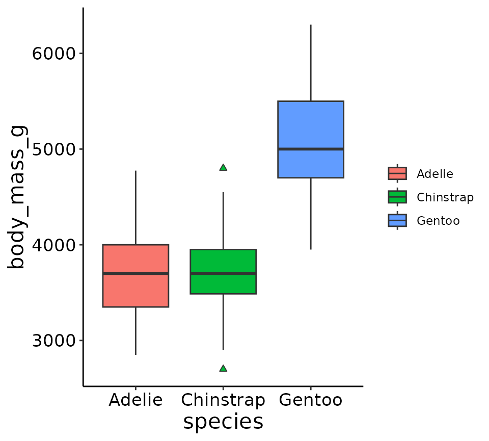
theme_lyon does the following changes to a
ggplot2 plot:
- Removes legend title and background
- Removes gray box behind colors in legend elements
- Removes major/minor gridlines
- Makes axes’ lines black
- Increases the font size of the axes titles and tick labels
# Load ggplot2
library(ggplot2)

# Create a plot and allow default ggplot themeing to be added
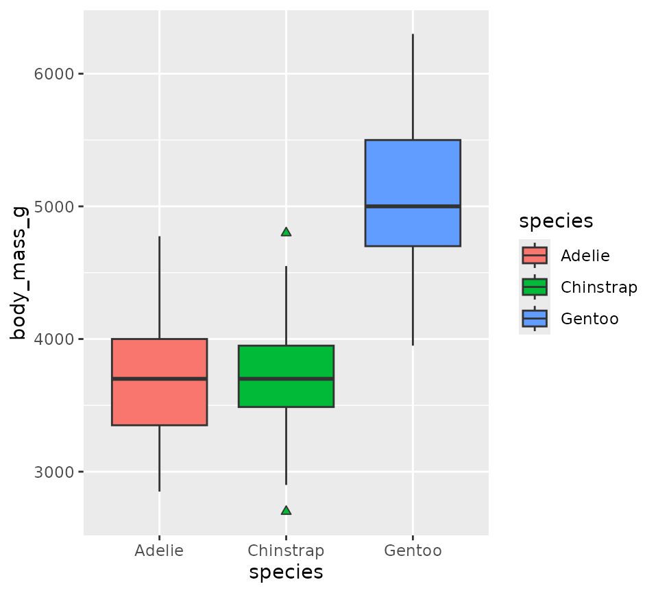
ggplot(penguins, aes(x = species, y = body_mass_g, fill = species)) +
  geom_boxplot(outlier.shape = 24)
# Compare with the same plot with my theme
ggplot(penguins, aes(x = species, y = body_mass_g, fill = species)) +
  geom_boxplot(outlier.shape = 24) +
  supportR::theme_lyon()
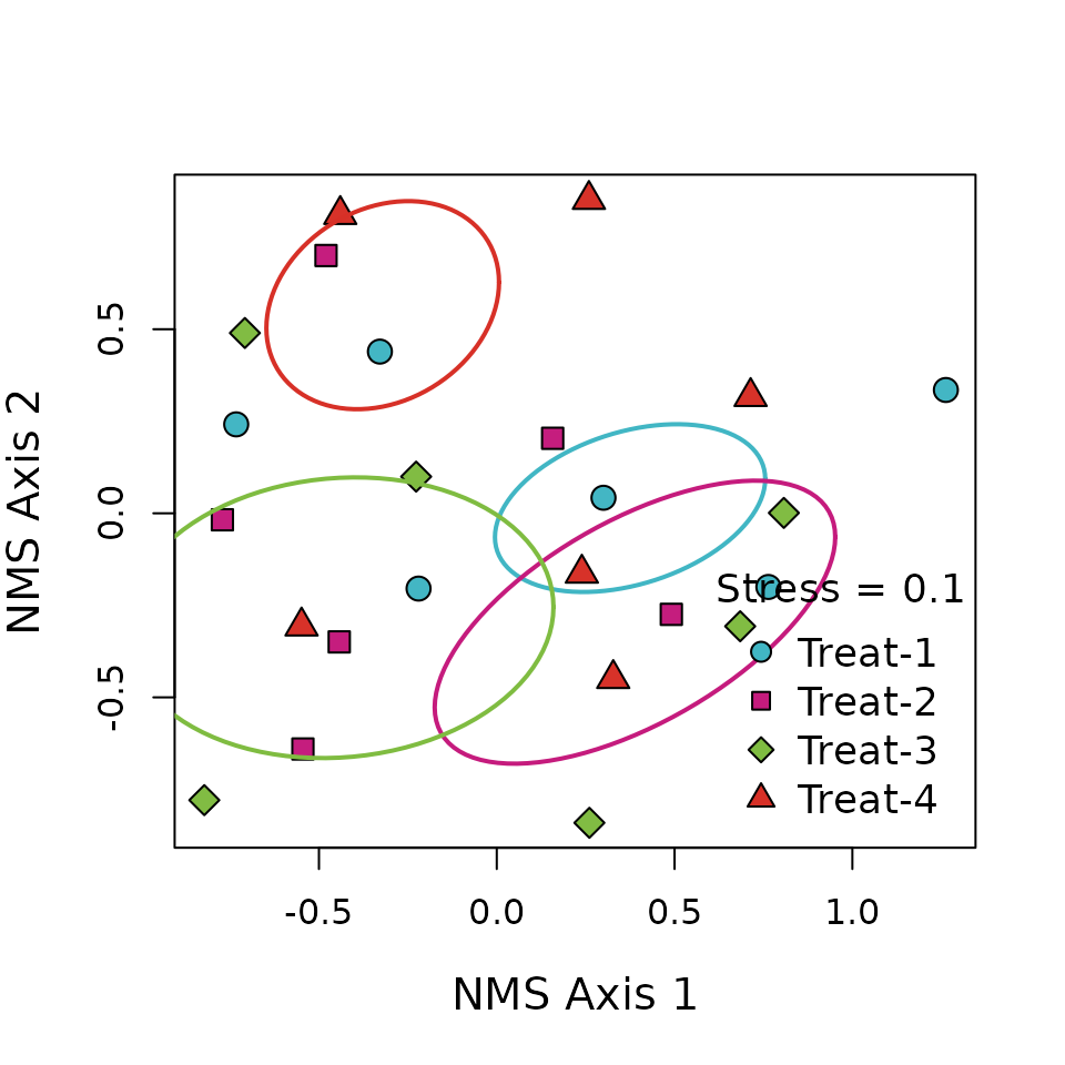
I’ve also created ordination for Nonmetric
Multidimensional Scaling (NMS) or Principal Coordinates Analysis (PCoA)
ordinations. Note that this function requires your multidimensional
scaling object be created by either ape::pcoa or
vegan::metaMDS.
# Load data from the `vegan` package
utils::data("varespec", package = "vegan")

# Make a columns to split the data into 4 groups
treatment <- c(rep.int("Trt_1", (nrow(varespec)/4)),
               rep.int("Trt_2", (nrow(varespec)/4)),
               rep.int("Trt_3", (nrow(varespec)/4)),
               rep.int("Trt_4", (nrow(varespec)/4)))

# And combine them into a single data object
data <- cbind(treatment, varespec)

# Actually perform multidimensional scaling
mds <- vegan::metaMDS(data[-1], autotransform = FALSE,
                      expand = FALSE, k = 2, try = 10)

# With the scaled object and original dataframe we can use this function
ordination(mod = mds, grps = data$treatment, x = "bottomright", legend = paste0("Treat-", 1:4))
Operations Outside of R
Finally, I’ve written several functions that allow you to interact with APIs outside of R via R functions with hopefully more comfortable syntax. Because these functions rely on user credentials, they cannot be run non-interactively (as in a CRAN submission) so the following code chunks are not evaluated and are included as examples of the proper syntax for your reference.
GitHub-Related Functions
For GitHub users, I’ve developed two related functions:
github_ls and github_tree.
github_ls accepts the URL to a GitHub repository to which
you have access (public or private). It creates a dataframe of that
repository’s contents including their names, types, and full paths
within the repository. Listing of a particular folder and recursive
listing of all nested subfolders within a repository are both supported
via additional arguments.
If the folder argument is set to NULL (the
default) the top level of the repository is listed.
# List all files in a GitHub repository
supportR::github_ls(repo = "https://github.com/njlyon0/supportR",
                    recursive = TRUE, quiet = FALSE)

# Or list files in only a particular folder
supportR::github_ls(repo = "https://github.com/njlyon0/supportR", folder = "R",
                    recursive = FALSE, quiet = TRUE)
github_tree is an extension of github_ls
that identifies all files in a repository and creates a file tree
diagram of that folder structure that is simple and human-readable.
Unlike github_ls, github_tree only supports
recursive identification of all files beginning at the top level of the
repository. It does however allow users to exclude the listings of
particular folders by specifying their names in the exclude
argument.
I think this could be particularly useful to embed in a repository’s
README.Rmd to create a quick-and-easy file map for visitors
to use as a guide in navigating the repository’s contents.
External File-Related Functions
Valuable information is sometimes stored as markdown files
which–while consistently formatted internally–are not always easily
parsed through R. I’ve written tabularize_md to ingest a
markdown file and collapse it into a table while still preserving the
nested structure of any headings that may be in the source file. This
function accepts either a local markdown file name/path or a connection
(via URL) to an online markdown file. I’ll demonstrate the URL-based
variant here but to use it on a local file you need only provide the
file name/path as you would to any other reading function (e.g.,
read.csv, etc.)
# Identify URL to the NEWS.md file in `supportR` GitHub repo
md_cxn <- url("https://raw.githubusercontent.com/njlyon0/supportR/main/NEWS.md")

# Transform it into a table
md_df <- tabularize_md(file = md_cxn)

# Close connection (just good housekeeping to do so)
close(md_cxn)

# Check out the table format
str(md_df)
Google Drive-Related Functions
For users who create RMarkdown reports and want to store them in a
Google Drive folder, rmd_export knits and exports a given R
Markdown file both locally and to a user-designated Google Drive folder.
Note that you MUST authenticate your R session
with the googledrive package so that it has permission to
access the Drive folder you supply. I recommend running
googledrive::drive_auth() and doing the authentication
“dance” in a browser before using rmd_export to reduce the
chances of any errors.
# Authorize R to interact with GoogleDrive
googledrive::drive_auth()

# Use `rmd_export()` to knit and export an .Rmd file
supportR::rmd_export(rmd = "my_markdown.Rmd",
                     in_path = file.path("Folder in my WD with the .Rmd named in `rmd`"),
                     out_path = file.path("Folder in my WD to save the knit file to"),
                     out_name = "desired name for output",
                     out_type = "html",
                     drive_link = "<Full Google Drive link>")