Multivariate Statistics 101

Nick J Lyon

Caveat Before We Begin

• Read this book

• Has a complete R appendix for:
  • Every example
  • Every figure
  • Every operation

• Essentially the book is written in R Markdown

• Bonus: actually pretty engaging to read!
  • Despite subject matter

Tutorial Outline

Background

Resampling & Permutation

Multivariate Data Visualization

Principle Components Analysis

Non-Metric Multidimensional Scaling

Multivariate Background

• Multivariate data have more variables (p) than observations (q)

• I.e., more columns than rows
  • True of most ecology/evolution datasets

• Differs from univariate statistics
  • Univariate explores variation in one variable
  • Multivariate explores variation in many variables (plus potential inter-relationships)

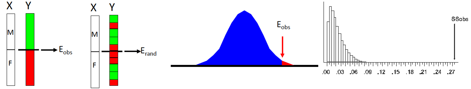
Resampling Methods

• Frequentist statistics uses distributions from theory

• Resampling statistics uses distributions from data

Theoretical Process

1. Take samples from data (i.e., “re-sample”)

2. Compare real observations to re-sampled groups

3. Evaluate significance

Permutation Notes

• Permutation methods are non-parametric
  • Because they don’t rely on a theoretical distribution

• Permutation methods are flexible
  • Can assess standard & non-standard experimental designs
  • Handle high-dimensional data (more variables than observations)

Two Major “Flavors”

Full Permutation

• Permute whole dataset

Residual Permutation

• Fit desired model
• Permute the residuals
  • Less sensitive to outliers

Multivariate Visualization

• Typically involves “ordination”

• Frequently uses “multidimensional scaling”
  • I.e., getting from many variables to fewer, more easily visualizable variables
  • Still representative of multivariate nature of data

• Common ordination methods include:
  • Principal Components Analysis (PCA)
  • Principal Coordinates Analysis (PCoA)
  • Nonmetric Multidimensional Scaling (NMS)

Principle Components Analysis

• Goal: reduce number of variables

• Mechanism: create combinations of existing variables to summarize variation
  • Want each combination to contain as much variation as possible
  • Such that you approach 100% variation summarized in only a few combinations

• Result: number of principal components equal to number of observations
  • Each principle component has a known % variation explained

PCA Process

• For variables (X_i) you want to create indices (I_k)

• Consider the following example:
  • I₁ = X₁ + X₂ + X₃ + X₄ + X₅
  • I₂ = X₁ - X₂ + X₃ + X₄ + X₅
  • I₃ = X₁ - X₂ - X₃ + X₄ + X₅
  • …
  • I_k = X₁ - X₂ - X₃ - X₄ - X₅

PCA Special Consideration 1

1. Axis orthogonality
   • Axes are “constrained to orthogonality” because of goal of maximized explained variation
   • Plain language: PC axes are perpendicular to one another

• Means PC₃ through PC_n are defined as soon as PC₁ and PC₂ are
  • Focusing on early PCs reduces the relevance of this issue

PCA Special Consideration 2

2. Not a hypothesis test

• PCA is great for visualizing patterns in data
  • Not good for statistical evaluation

• I.e., PCA cannot–by itself–show support for your hypothesis

Nonmetric Multidimensional Scaling

• Goal: reduce number of variables
  • Same as PCA!

• Mechanism: scale dissimilarity of points to minimize “stress”
  • “dissimilarity” != “distance”
  • Stress is a metric for tension between true spatial configuration of points versus the arrangement of their dissimilarity

• Result: number of NMS axes is defined by the user
  • NMS reports stress of “best” solution (essentially a goodness of fit metric)

NMS Process

1. Choose a starting configuration of points (randomly)

2. Move points around and measure stress at each configuration

3. Repeat until stress has been minimized

4. Return to step 1 with different starting points
   • Necessary to avoid local stress minima

5. Continue 1-4 until confident true minimum stress configuration has been found

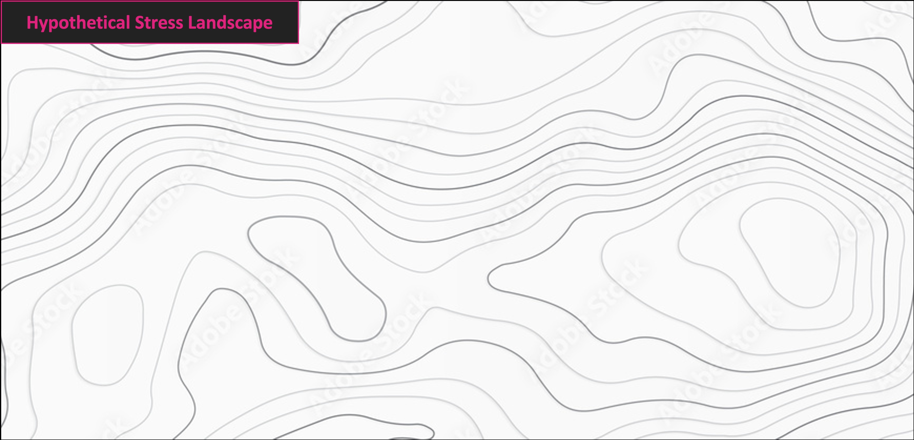
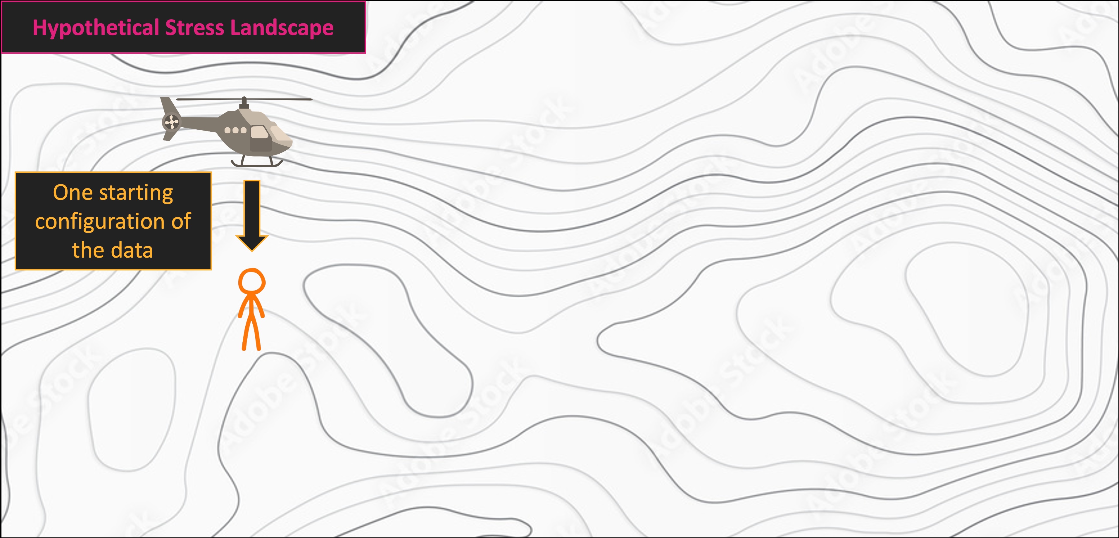
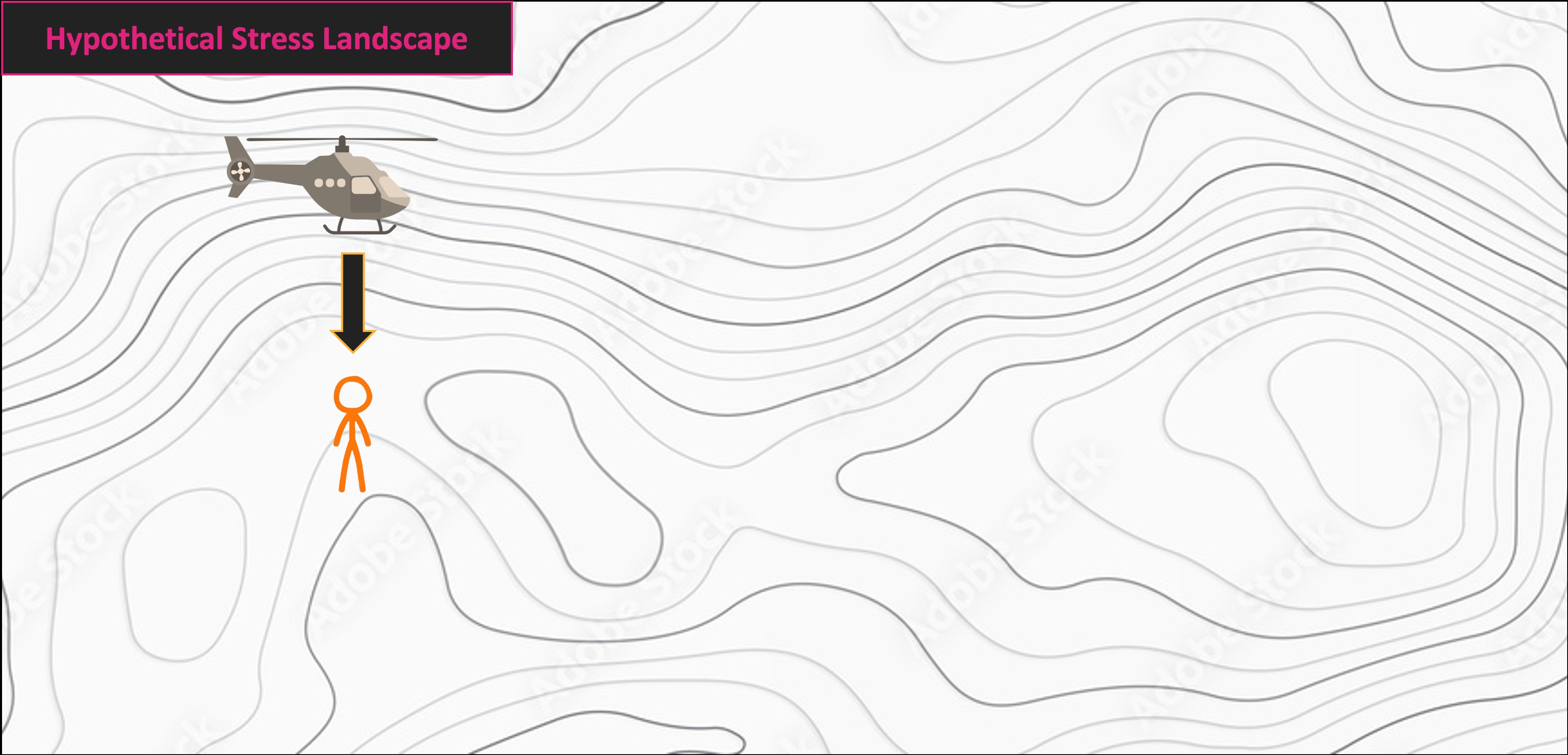
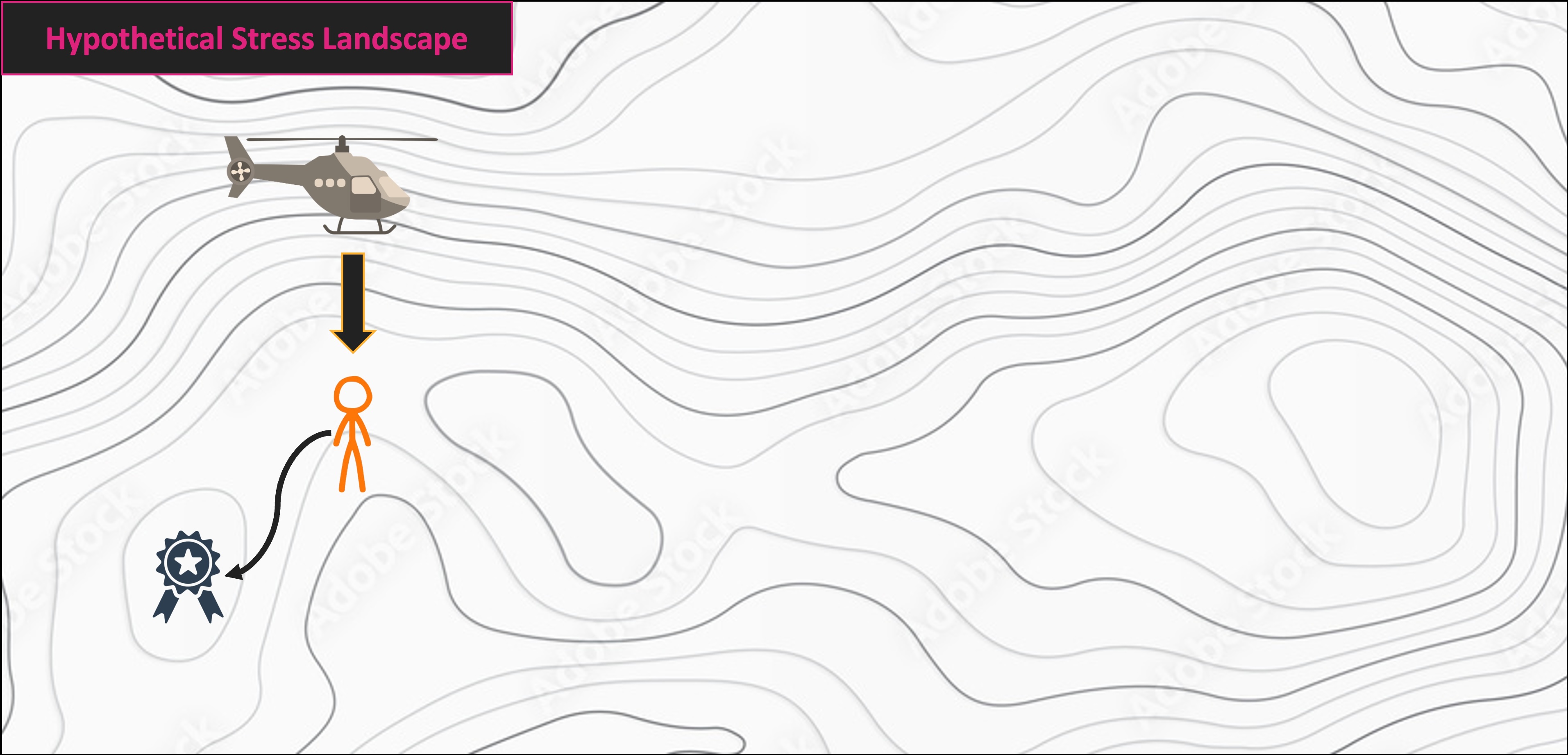
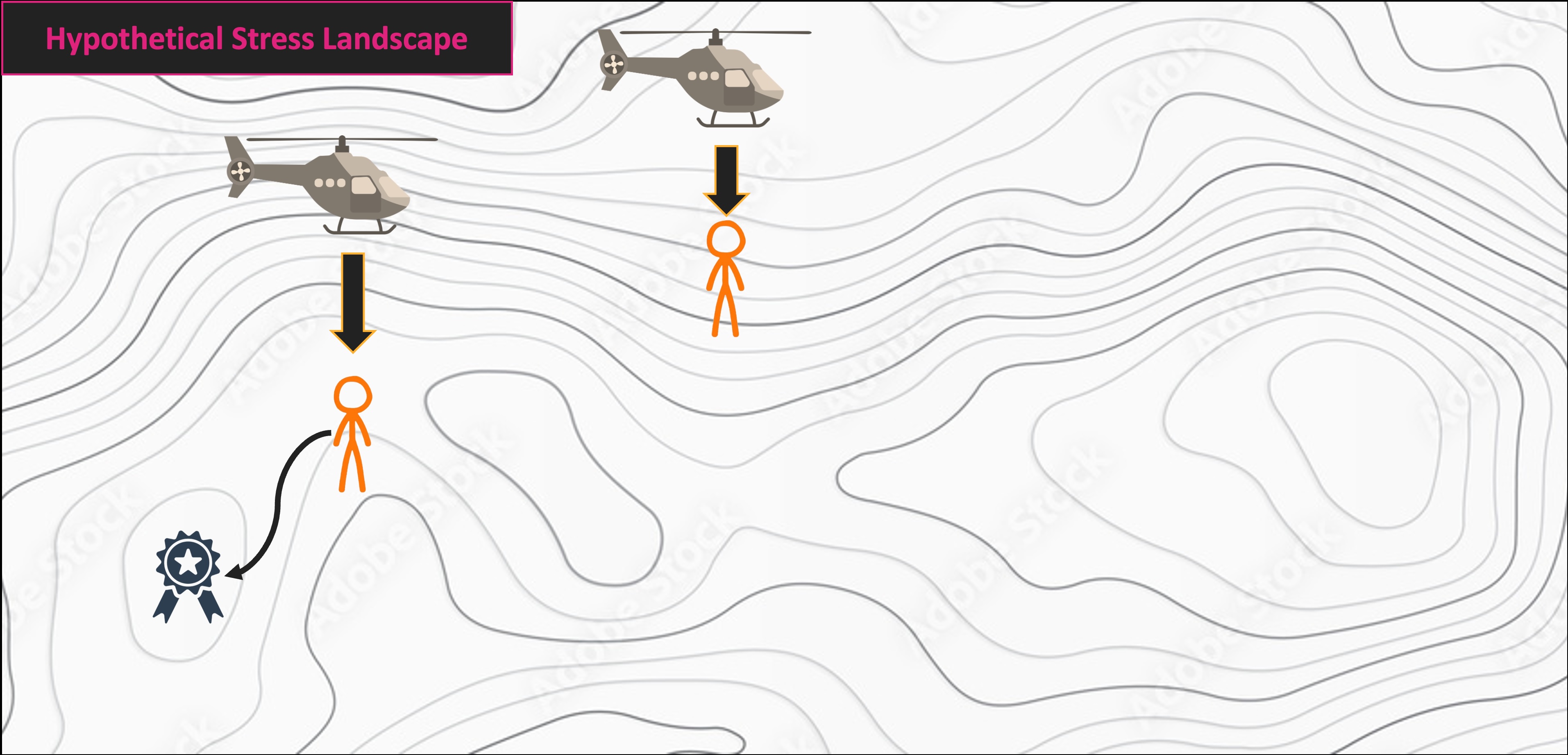
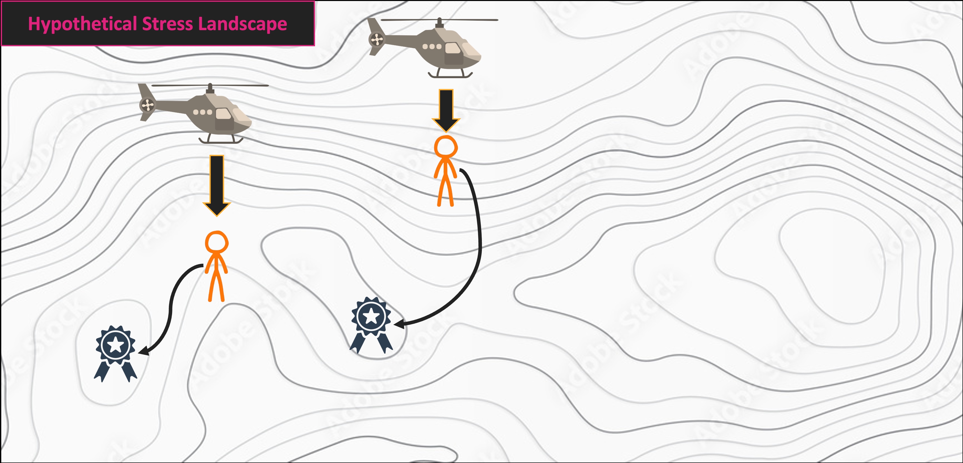
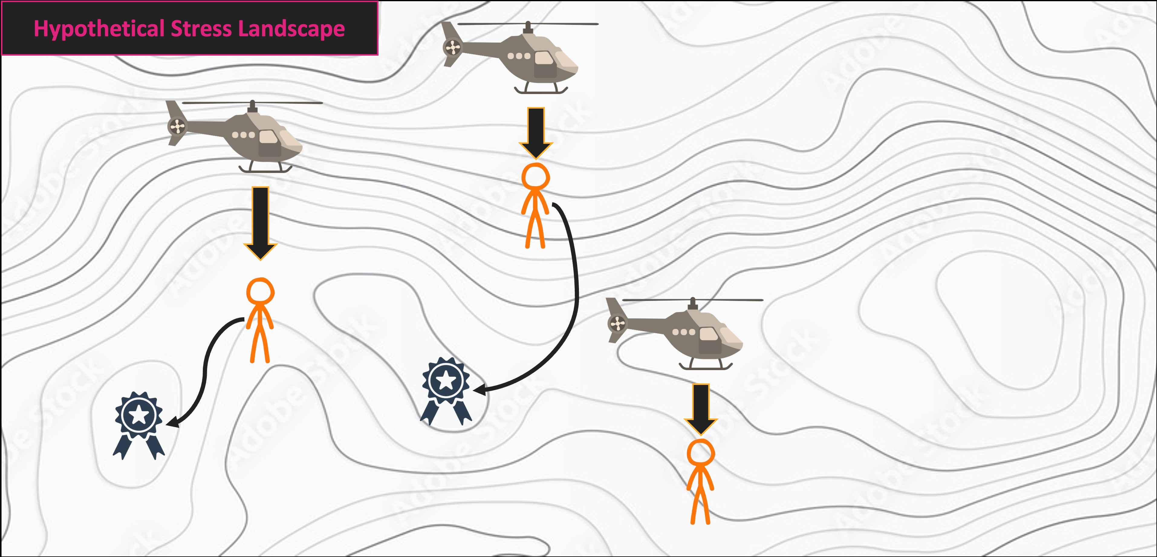
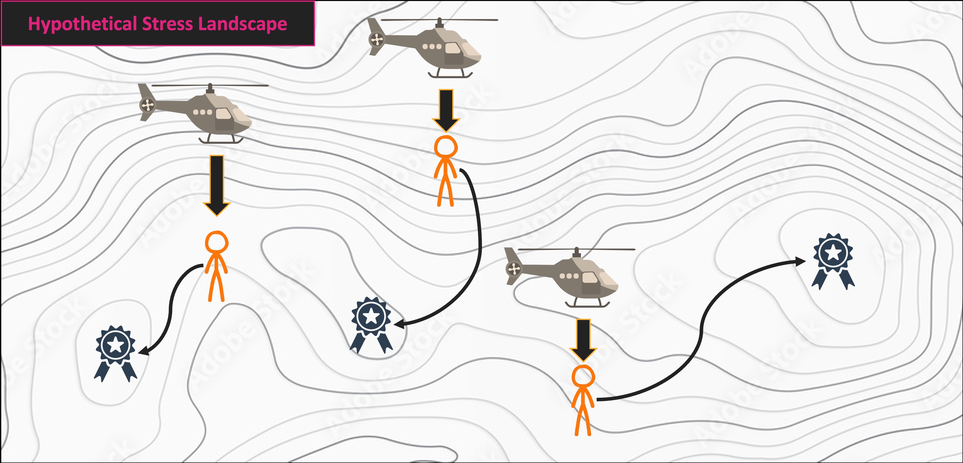
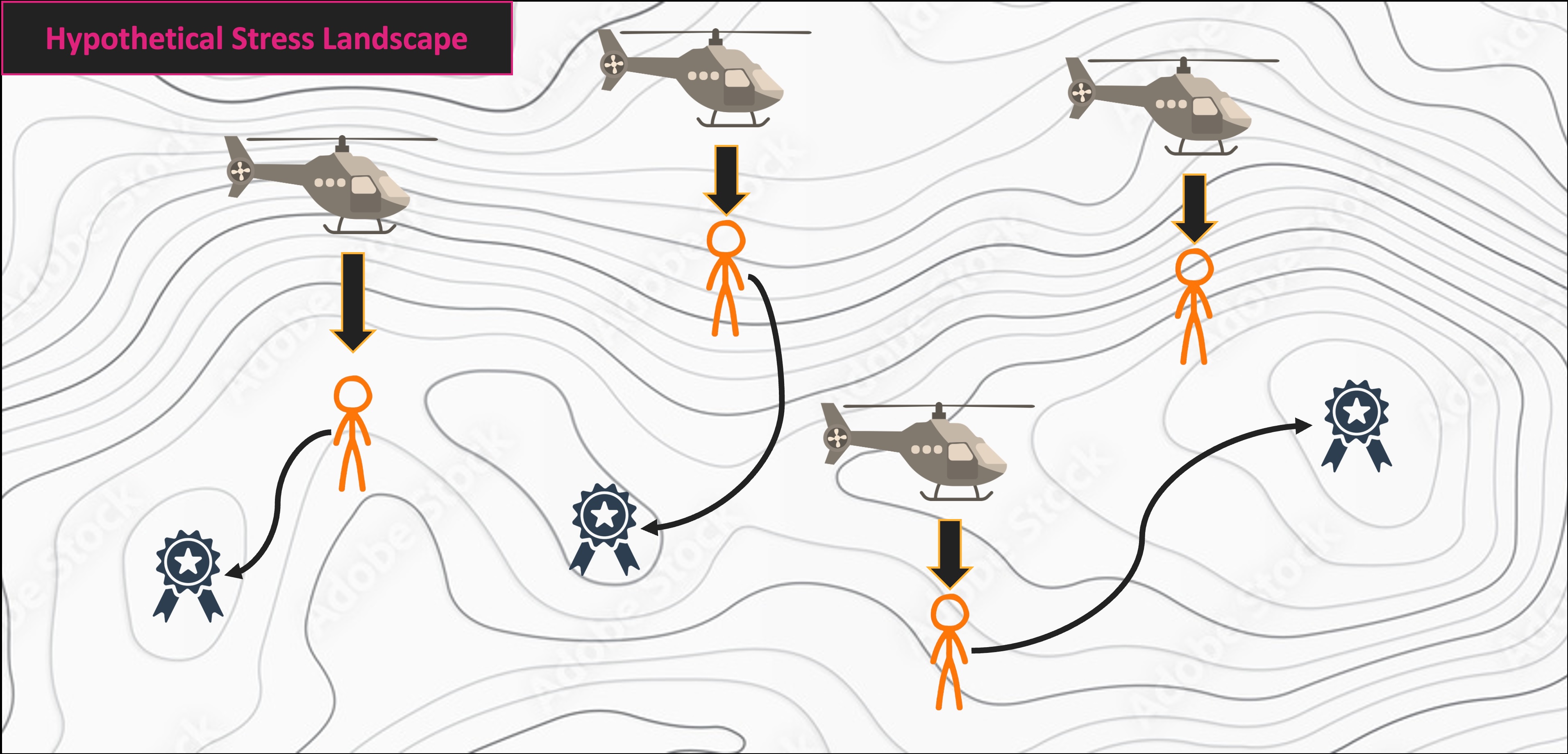
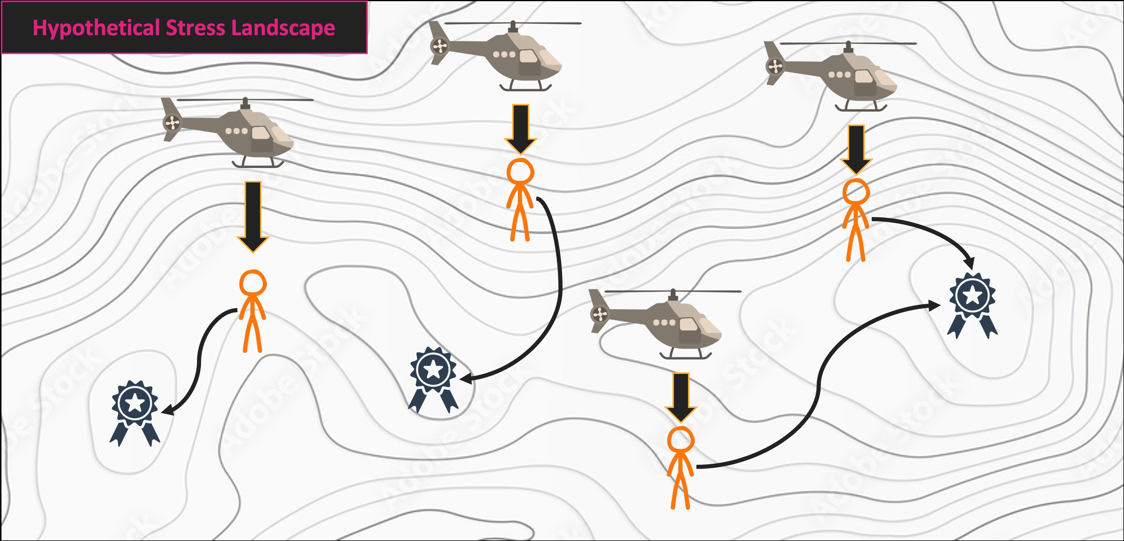
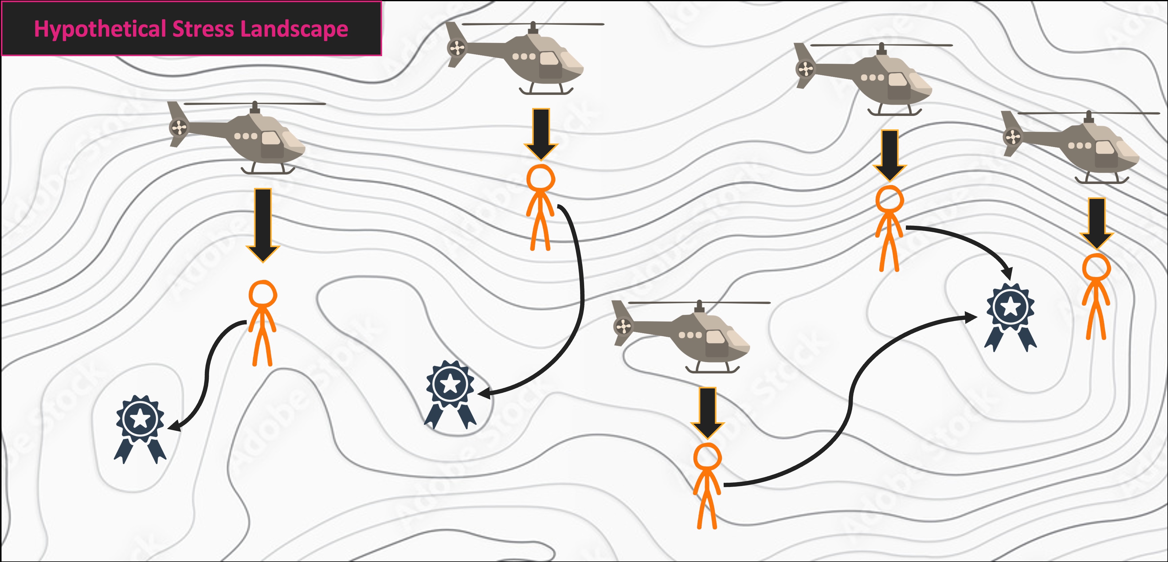
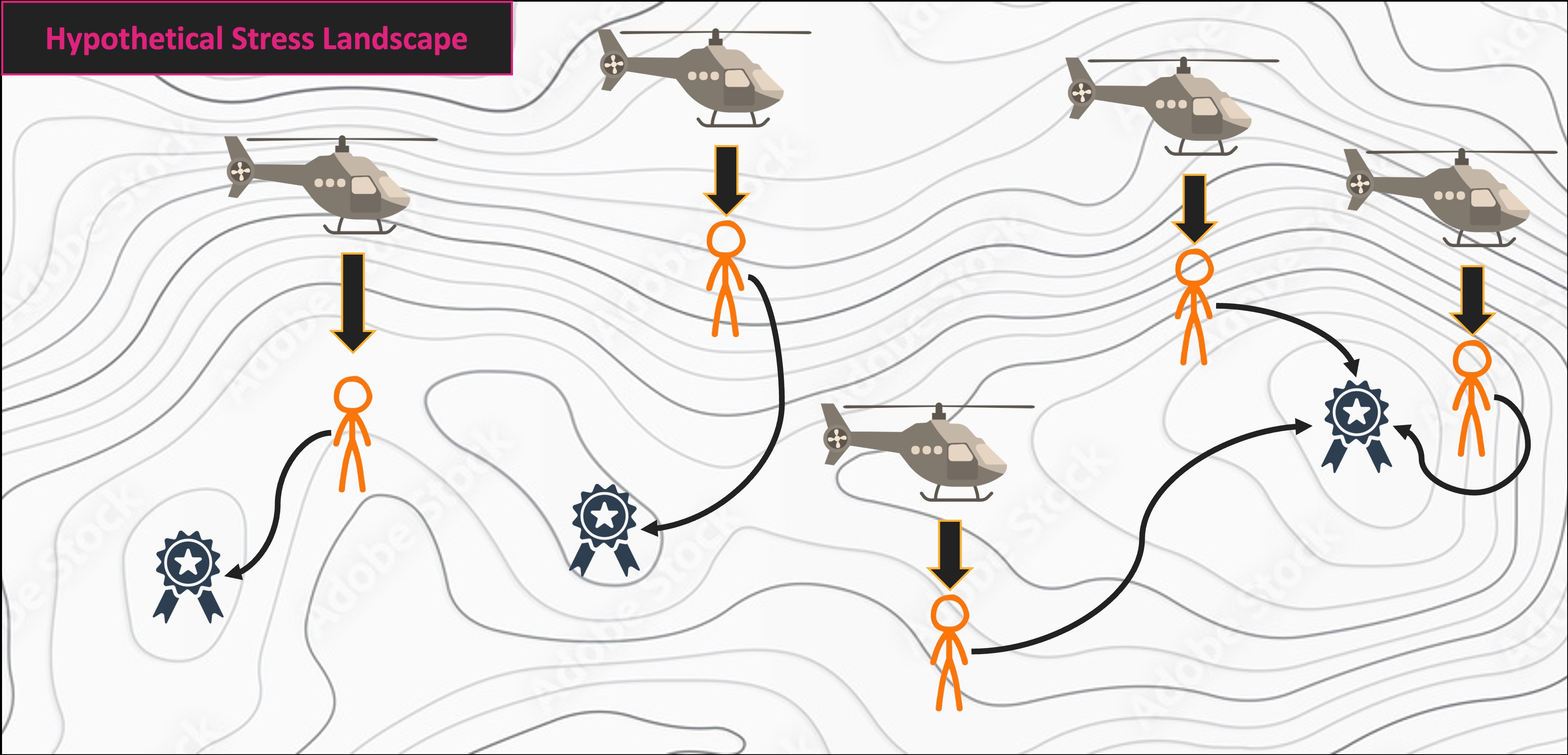
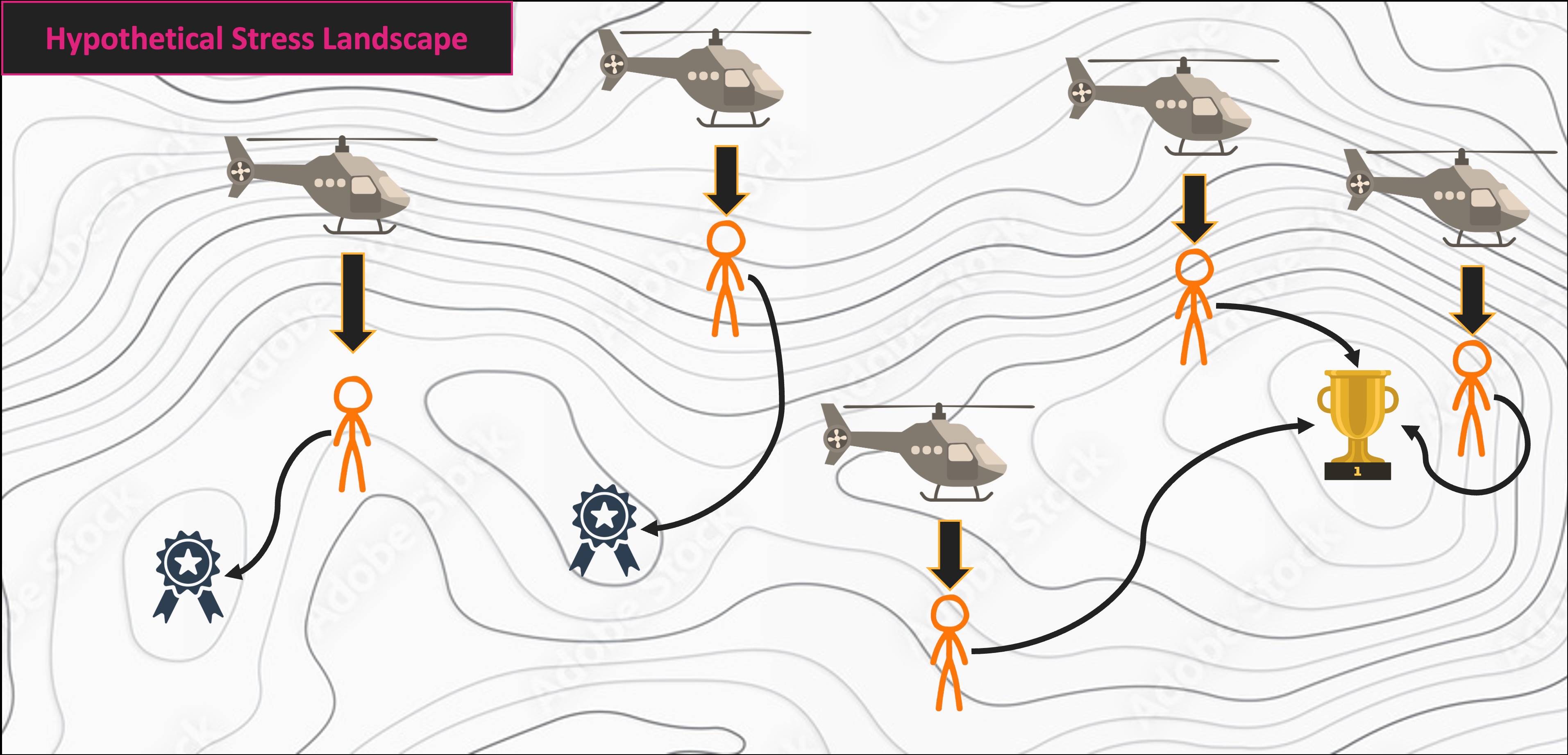
NMS Helicopter Analogy

Multivariate Code Demo

Prepare

• First, you’ll need to install and load a few R packages
  • While not technically necessary, the librarian package makes library management much simpler

# Install librarian (if you need to)
# install.packages("librarian")

# Install (if not already present) and load needed libraries
librarian::shelf(vegan, RRPP, scatterplot3d, TeachingDemos, supportR)

Lichen Data

• The vegan package includes some lichen community composition data we can use for exploratory purposes

• We’ll begin by loading that and creating artificial groups for later analysis

# Load vegan's lichen dataset
utils::data("varespec", package = 'vegan')

# Make some columns of known number of groups
treatment <- c(rep.int("Trt1", (nrow(varespec)/4)),
               rep.int("Trt2", (nrow(varespec)/4)),
               rep.int("Trt3", (nrow(varespec)/4)),
               rep.int("Trt4", (nrow(varespec)/4)))

# And combine them into a single data object
lichen_df <- cbind(treatment, varespec)

Data Structure

• This data object now has the following structure:

# Check lichen data structure
str(lichen_df)

'data.frame':   24 obs. of  45 variables:
 $ treatment: chr  "Trt1" "Trt1" "Trt1" "Trt1" ...
 $ Callvulg : num  0.55 0.67 0.1 0 0 ...
 $ Empenigr : num  11.13 0.17 1.55 15.13 12.68 ...
 $ Rhodtome : num  0 0 0 2.42 0 0 1.55 0 0.35 0.07 ...
 $ Vaccmyrt : num  0 0.35 0 5.92 0 ...
 $ Vaccviti : num  17.8 12.1 13.5 16 23.7 ...
 $ Pinusylv : num  0.07 0.12 0.25 0 0.03 0.12 0.1 0.1 0.05 0.12 ...
 $ Descflex : num  0 0 0 3.7 0 0.02 0.78 0 0.4 0 ...
 $ Betupube : num  0 0 0 0 0 0 0.02 0 0 0 ...
 $ Vacculig : num  1.6 0 0 1.12 0 0 2 0 0.2 0 ...
 $ Diphcomp : num  2.07 0 0 0 0 0 0 0 0 0.07 ...
 $ Dicrsp   : num  0 0.33 23.43 0 0 ...
 $ Dicrfusc : num  1.62 10.92 0 3.63 3.42 ...
 $ Dicrpoly : num  0 0.02 1.68 0 0.02 0.02 0 0.23 0.2 0 ...
 $ Hylosple : num  0 0 0 6.7 0 0 0 0 9.97 0 ...
 $ Pleuschr : num  4.67 37.75 32.92 58.07 19.42 ...
 $ Polypili : num  0.02 0.02 0 0 0.02 0.02 0 0 0 0 ...
 $ Polyjuni : num  0.13 0.23 0.23 0 2.12 1.58 0 0.02 0.08 0.02 ...
 $ Polycomm : num  0 0 0 0.13 0 0.18 0 0 0 0 ...
 $ Pohlnuta : num  0.13 0.03 0.32 0.02 0.17 0.07 0.1 0.13 0.07 0.03 ...
 $ Ptilcili : num  0.12 0.02 0.03 0.08 1.8 0.27 0.03 0.1 0.03 0.25 ...
 $ Barbhatc : num  0 0 0 0.08 0.02 0.02 0 0 0 0.07 ...
 $ Cladarbu : num  21.73 12.05 3.58 1.42 9.08 ...
 $ Cladrang : num  21.47 8.13 5.52 7.63 9.22 ...
 $ Cladstel : num  3.5 0.18 0.07 2.55 0.05 ...
 $ Cladunci : num  0.3 2.65 8.93 0.15 0.73 0.25 2.38 0.82 0.05 0.95 ...
 $ Cladcocc : num  0.18 0.13 0 0 0.08 0.1 0.17 0.15 0.02 0.17 ...
 $ Cladcorn : num  0.23 0.18 0.2 0.38 1.42 0.25 0.13 0.05 0.03 0.05 ...
 $ Cladgrac : num  0.25 0.23 0.48 0.12 0.5 0.18 0.18 0.22 0.07 0.23 ...
 $ Cladfimb : num  0.25 0.25 0 0.1 0.17 0.1 0.2 0.22 0.1 0.18 ...
 $ Cladcris : num  0.23 1.23 0.07 0.03 1.78 0.12 0.2 0.17 0.02 0.57 ...
 $ Cladchlo : num  0 0 0.1 0 0.05 0.05 0.02 0 0 0.02 ...
 $ Cladbotr : num  0 0 0.02 0.02 0.05 0.02 0 0 0.02 0.07 ...
 $ Cladamau : num  0.08 0 0 0 0 0 0 0 0 0 ...
 $ Cladsp   : num  0.02 0 0 0.02 0 0 0.02 0.02 0 0.07 ...
 $ Cetreric : num  0.02 0.15 0.78 0 0 0 0.02 0.18 0 0.18 ...
 $ Cetrisla : num  0 0.03 0.12 0 0 0 0 0.08 0.02 0.02 ...
 $ Flavniva : num  0.12 0 0 0 0.02 0.02 0 0 0 0 ...
 $ Nepharct : num  0.02 0 0 0 0 0 0 0 0 0 ...
 $ Stersp   : num  0.62 0.85 0.03 0 1.58 0.28 0 0.03 0.02 0.03 ...
 $ Peltapht : num  0.02 0 0 0.07 0.33 0 0 0 0 0.02 ...
 $ Icmaeric : num  0 0 0 0 0 0 0 0.07 0 0 ...
 $ Cladcerv : num  0 0 0 0 0 0 0 0 0 0 ...
 $ Claddefo : num  0.25 1 0.33 0.15 1.97 0.37 0.15 0.67 0.08 0.47 ...
 $ Cladphyl : num  0 0 0 0 0 0 0 0 0 0 ...

• Each column is an abbreviated lichen species name and the values are % cover

Permutation Analysis

• First, we’ll use the RRPP package to use permutation analysis
  • H_A: lichen community composition differs between at least two groups
  • H₀: lichen community composition does not differ

• Note that RRPP does require a special class of data object to perform analysis

# Make the special data object class required by RRPP
lichen_rpdf <- RRPP::rrpp.data.frame("community" = as.matrix(varespec),
                                     "treatment" = lichen_df$treatment)

# Fit permutation model
lich_fit <- RRPP::lm.rrpp(community ~ treatment, data = lichen_rpdf, iter = 999, RRPP = T)

• Quick argument explanation:
  • The iter argument is the number of permutations
  • The RRPP argument is whether to permute residuals (TRUE) or the full data (FALSE)

Permutation Analysis Results

• To check the results, we can use the anova function
  • This also allows us to specify the desired effect type

# Check out the results of the analysis!
RRPP::anova.lm.rrpp(lich_fit, effect.type = "F", print.progress = F)

Analysis of Variance, using Residual Randomization
Permutation procedure: Randomization of null model residuals 
Number of permutations: 1000 
Estimation method: Ordinary Least Squares 
Sums of Squares and Cross-products: Type I 
Effect sizes (Z) based on F distributions

          Df    SS     MS     Rsq      F     Z Pr(>F)    
treatment  3 19602 6533.9 0.46682 5.8369 3.655  0.001 ***
Residuals 20 22388 1119.4 0.53318                        
Total     23 41990                                       
---
Signif. codes:  0 '***' 0.001 '**' 0.01 '*' 0.05 '.' 0.1 ' ' 1

Call: RRPP::lm.rrpp(f1 = community ~ treatment, iter = 999, RRPP = T,  
    data = lichen_rpdf)

• Now we get a fairly standard ANOVA table
  • The Z column is the “Z score” and is essentially the effect size

Permutation Pairwise Comparisons

• Once we have our main results, we can also get pairwise comparison results

# Perform pairwise comparisons
lich_pairs <- RRPP::pairwise(fit = lich_fit, groups = treatment)

# Check results
summary(lich_pairs)

Pairwise comparisons

Groups: Trt1 Trt2 Trt3 Trt4 

RRPP: 1000 permutations

LS means:
Vectors hidden (use show.vectors = TRUE to view)

Pairwise distances between means, plus statistics
                 d UCL (95%)          Z Pr > d
Trt1:Trt2 16.48128  39.64863 -0.7289177  0.760
Trt1:Trt3 38.04299  40.10757  1.5478150  0.067
Trt1:Trt4 59.41369  38.99550  2.9255939  0.001
Trt2:Trt3 37.15261  38.01919  1.5148939  0.063
Trt2:Trt4 62.40360  39.28595  3.0093479  0.001
Trt3:Trt4 50.44284  40.37863  2.2553908  0.005

• These show that the fourth treatment significantly differs from the other three
  • And the third marginally differs from the first and second

Multivariate Data Visualization

• There are a few non-ordination ways of doing multivariate visualization
  • Note that these are mostly for exploratory purposes

• They’re still helpful for checking the general ‘vibe’ of the data
  • but they may not hold up to formal review processes

3D Scatterplot

• Perhaps the simplest mode of multivariate data visualization is just to make a 3D scatterplot!
  • Still technically counts as “multivariate” visualization

• Primary benefit is that interpretation is pretty straightforward

# Make 3D scatterplot with `scatterplot3d` library
scatterplot3d::scatterplot3d(lichen_df$Callvulg, lichen_df$Empenigr, lichen_df$Rhodtome,
                     xlab = "Callvulg", ylab = "Empenigr", zlab = "Rhodtome")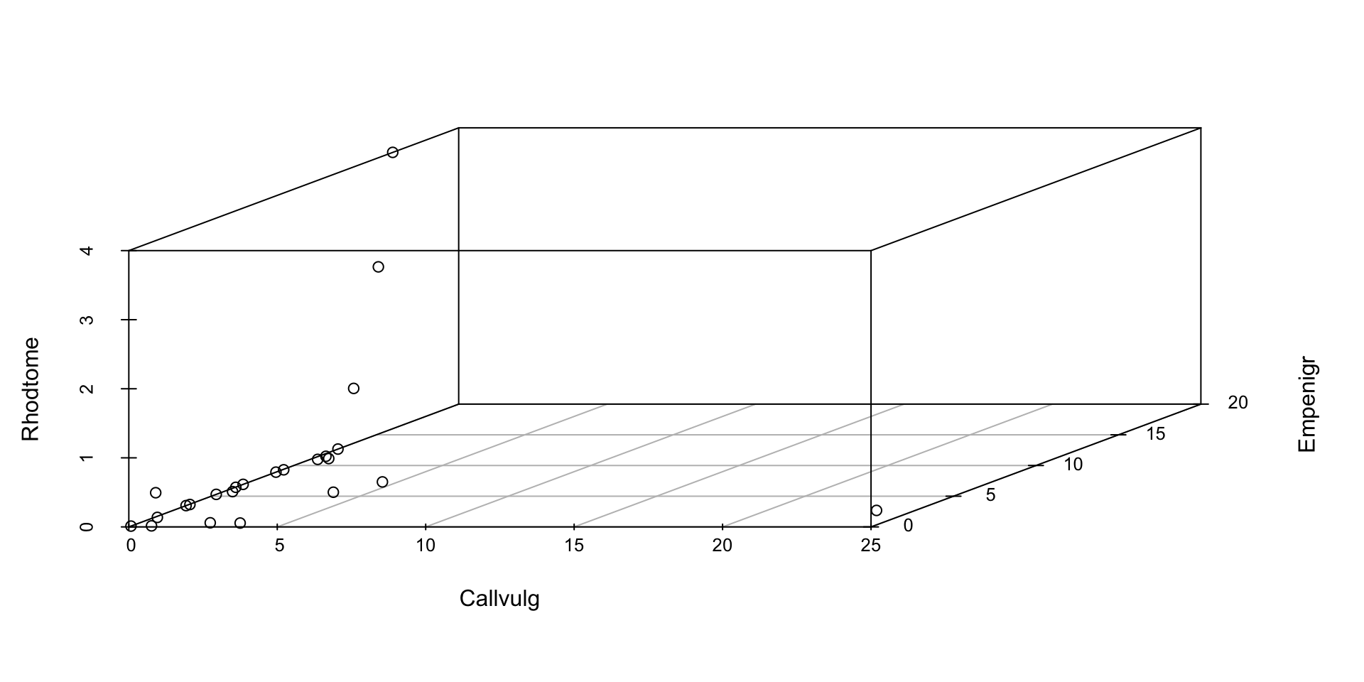

Chernoff Faces

• Some people have tried to make human’s capacity for comparing faces into a tool for data visualization
  • Data are transformed into human(-ish) faces with different dimensions
  • I find these very scary

# Make a matrix out of your desired data
lich_mat <- data.matrix(varespec)

# Generate Chernoff face graph
TeachingDemos::faces2(lich_mat, labels = lichen_df$treatment, scale = "center")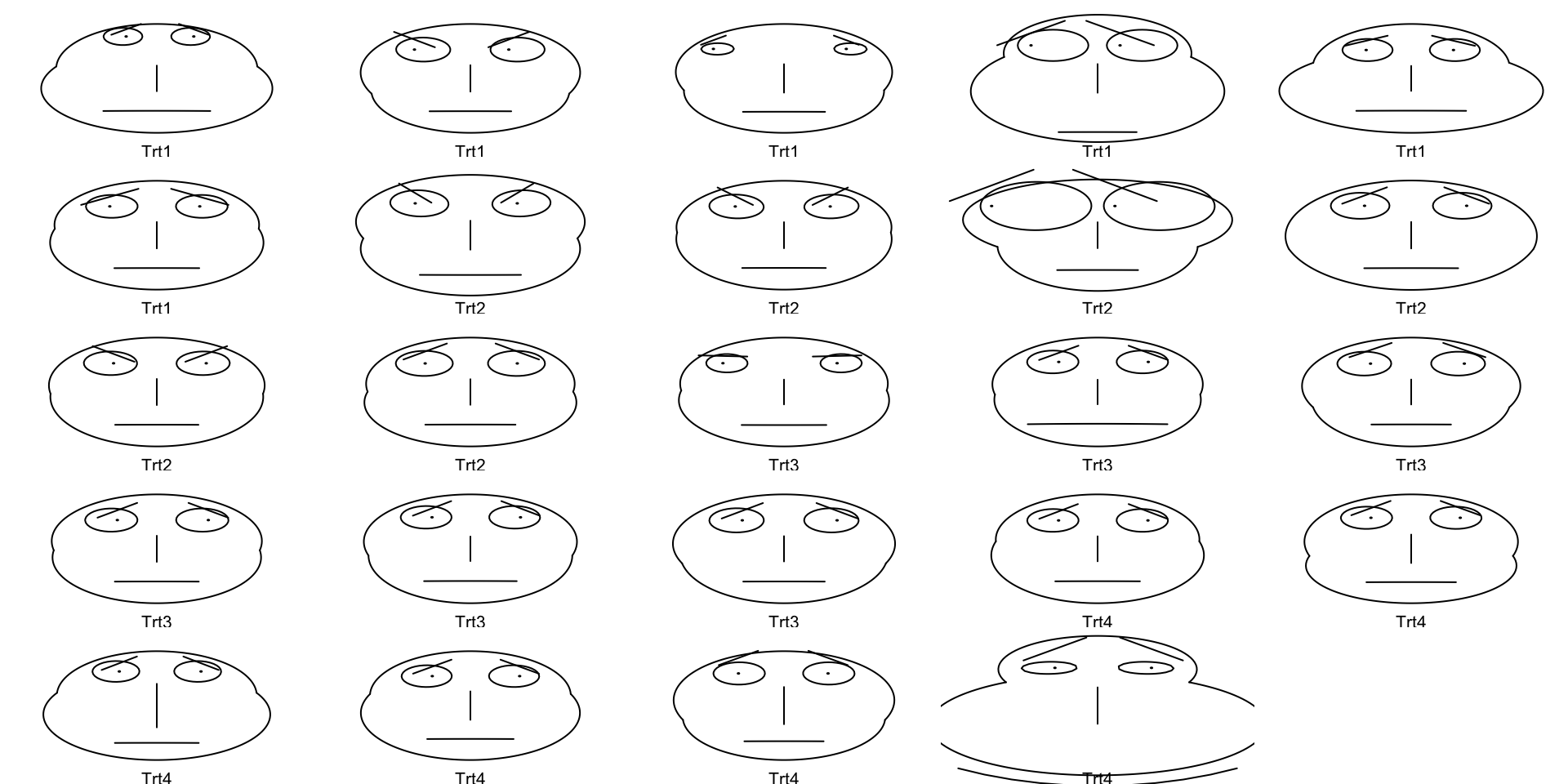

Star Plots

• Perhaps most usefully, you can just make “star plots” to check multivariate data

# Create star plots
graphics::stars(x = varespec, labels = lichen_df$treatment, key.loc = c(16, 9))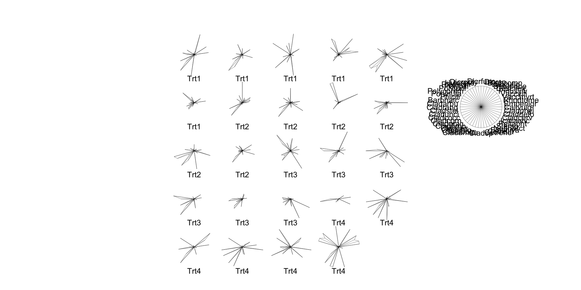

Principal Components

• Before we can visualize PCA results, we need to actually identify PC axes!

# Perform Principal Components Analysis
lich_pc <- prcomp(x = varespec)

# Summarize it to calculate '% variation explained' for each PC axis
lich_pc_smry <- summary(lich_pc)

# Check the structure of the summarized object
str(lich_pc_smry)

List of 6
 $ sdev      : num [1:24] 31.35 21.55 11.5 8.6 6.96 ...
 $ rotation  : num [1:44, 1:24] -0.01399 0.01566 -0.00646 -0.05168 0.00858 ...
  ..- attr(*, "dimnames")=List of 2
  .. ..$ : chr [1:44] "Callvulg" "Empenigr" "Rhodtome" "Vaccmyrt" ...
  .. ..$ : chr [1:24] "PC1" "PC2" "PC3" "PC4" ...
 $ center    : Named num [1:44] 1.88 6.33 0.35 2.11 11.46 ...
  ..- attr(*, "names")= chr [1:44] "Callvulg" "Empenigr" "Rhodtome" "Vaccmyrt" ...
 $ scale     : logi FALSE
 $ x         : num [1:24, 1:24] -10.8 -27.8 -25.7 -31.8 -19.6 ...
  ..- attr(*, "dimnames")=List of 2
  .. ..$ : chr [1:24] "18" "15" "24" "27" ...
  .. ..$ : chr [1:24] "PC1" "PC2" "PC3" "PC4" ...
 $ importance: num [1:3, 1:24] 31.352 0.538 0.538 21.548 0.254 ...
  ..- attr(*, "dimnames")=List of 2
  .. ..$ : chr [1:3] "Standard deviation" "Proportion of Variance" "Cumulative Proportion"
  .. ..$ : chr [1:24] "PC1" "PC2" "PC3" "PC4" ...
 - attr(*, "class")= chr "summary.prcomp"

Principal Components Ordination

# With that done, we can make a graph of that information!
plot(x = lich_pc$x[,1], y = lich_pc$x[,2], pch = 20, 
     ## And do some fancy axis labels to get 'variation explained' in the plot
     xlab = paste0("PC1 (", (lich_pc_smry$importance[2, 1] * 100), " % variation explained)"), 
     ylab = paste0("PC2 (", (lich_pc_smry$importance[2, 2] * 100), " % variation explained)"))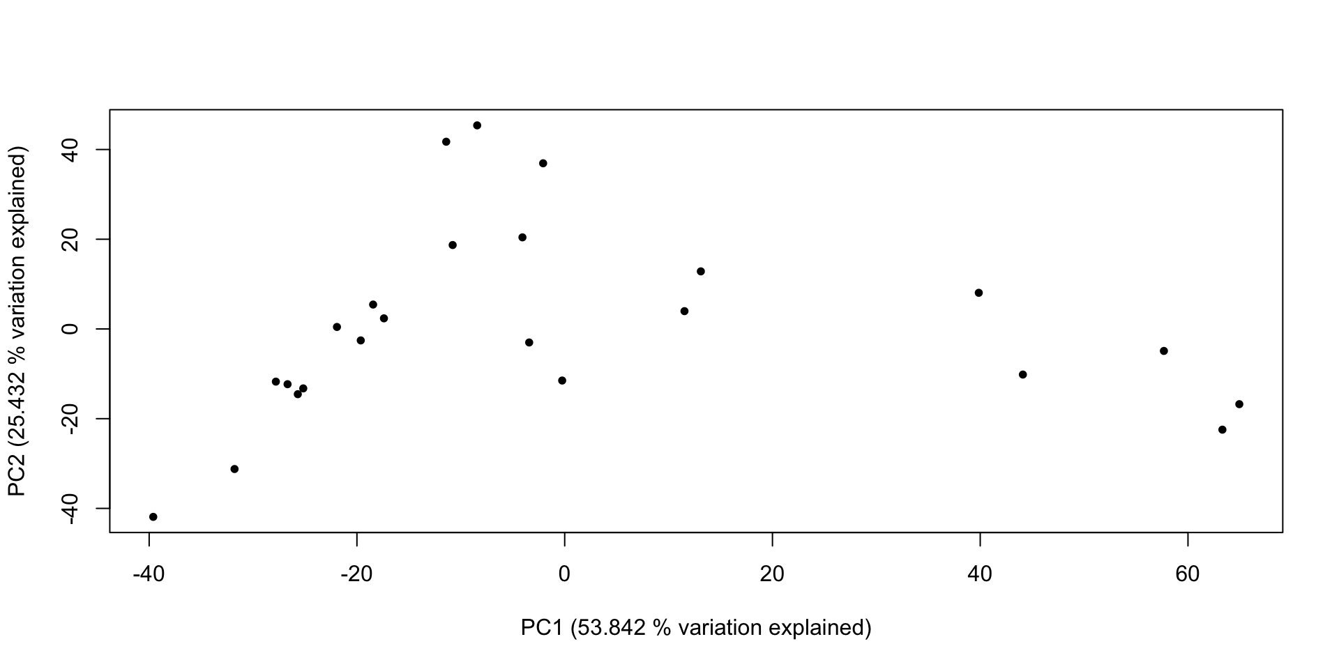

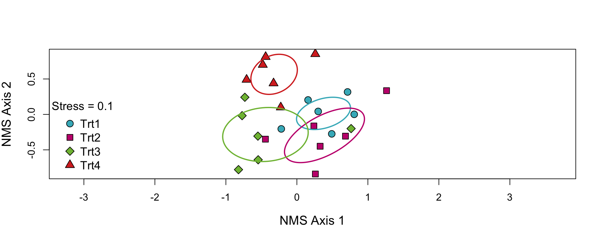
Non-Metric Multidimensional Scaling

• Just like PCA, we need to start by actually performing the scaling step

• See here:

# Perform NMS ordination
lich_mds <- vegan::metaMDS(comm = varespec, distance = "bray", k = 2, try = 50,
                           autotransform = F, expand = F)

• Quick explanation of (some of) the arguments
  • distance is your preferred metric for dissimilarity
  • k is the number of axes to scale to (typically 2 for standard plotting)
  • try is the number of starting data configurations (remember the helicopter analogy!)

NMS Ordination

• Fortunately, we can use a nice ordination function from the supportR package to make the graph

# Create NMS ordination
supportR::nms_ord(mod = lich_mds, groupcol = lichen_df$treatment)

Thanks! Questions?