Intro to Data Science

Lecture 5 – Multi-Model Inference

A Guide to Your Process

Scheduling

Learning Objectives

Practice

Supporting Information

Class Discussion

Today’s Plan

• Interactions
• Multi-Model Inference
• Mid-Term Instructor Evaluations
• Free Work on Function Tutorials

Today’s Learning Objectives

After today’s session you will be able to:

• Perform more analytical tests using R
• Explain an “interaction term” in the context of life sciences
• Compare model strengths in R

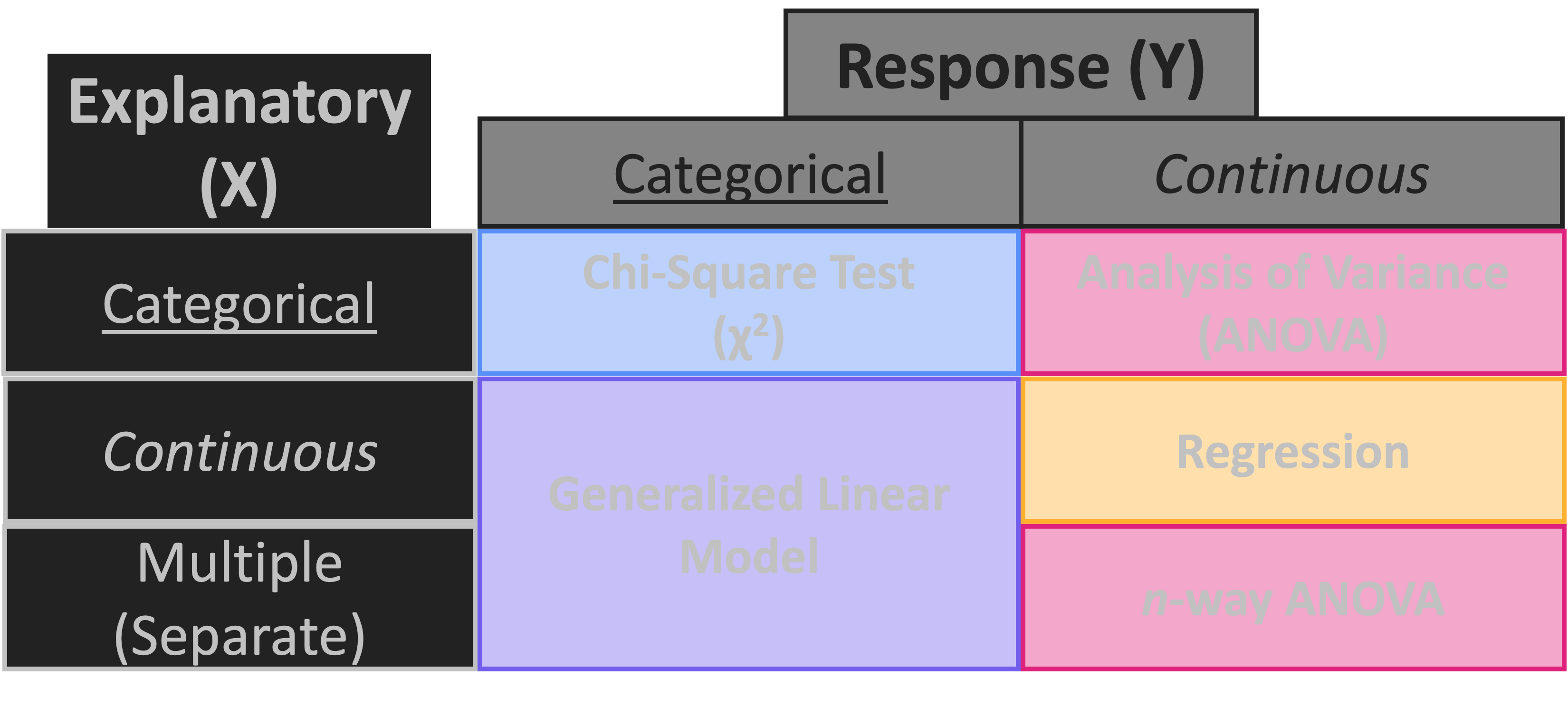
Roadmap Reminder

Interaction Terms

• So far, we’ve assumed the effect on Y is due to each X separately
  • In real life, the effect on Y may be due to interactions among X variables!

• Arguably, all of biology lives in these interactions!

Interactions Examples

• Let’s consider some examples to hopefully make this “click” for you

1. The number of ant hills (Y) depends on both how hot it is (X) and how rainy it is (X)

2. Raccoons are fatter (Y) when they live close to humans (X) and the weather is mild (X)

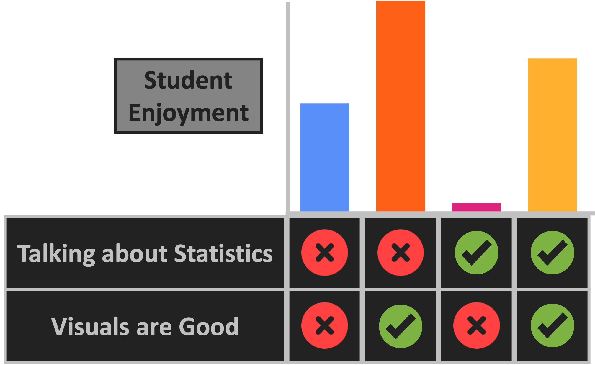
Interaction Visual

• One more example:
  • Students enjoy (Y) talking about stats (X) if there are good visuals (X)

Roadmap Extension: Interactions

R Syntax for Interactions

• Two ways to add additional an interaction between two explanatory variables:
  • Use an asterisk (*) between the two terms
  • Use a colon (:)

• Using an asterisk includes both terms separately and their interaction

• Example syntax:

# Use the asterisk to test an interaction
stat_test(response ~ exp1 * exp2, data = my_df)

# Fit the SAME MODEL with a colon instead
stat_test(response ~ exp1 + exp2 + exp1:exp2, data = my_df)

Analysis of Co-Variance (ANCOVA)

• Multiple X variables and Y is continuous
  • X variables may be either categorical or continuous
  • Must also include an “interaction term” between (at least) two of the X variables

• Hypothesis: The effect on Y is due to the interaction of X variables
  • H₀: The effect on Y is not due to interactions among X variables

• Returns a P value for the interaction term and each X variable separately

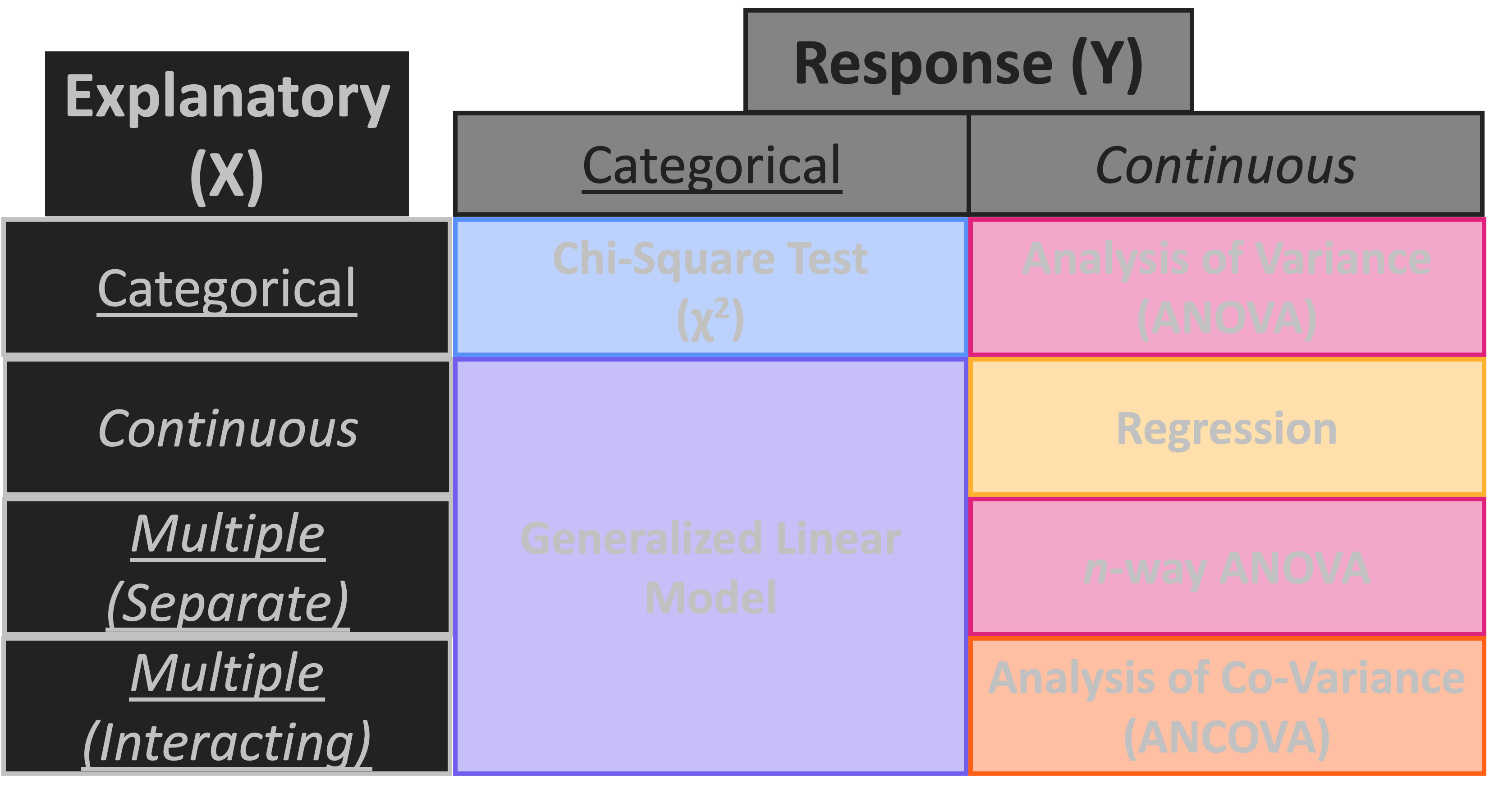
Practice: ANCOVA

• ANCOVA function is the same as the regular ANOVA / n-way ANOVA – aov

• New penguin-related hypothesis:
  • H_A: Penguin body mass differs among species and within a species between sexes
  • H₀: Sex-specific differences on penguin body mass are not species-dependent

• Test H_A with an interaction term!
  • Was your hypothesis supported?
  • What difference(s) do you see between this and a 2-way ANOVA summary table?

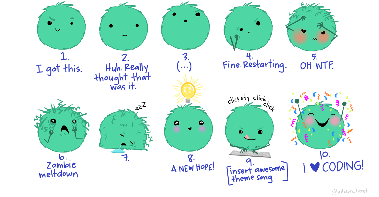
Temperature Check

How are you Feeling?

Discussion: Null Hypothesis Testing

• What lingering questions do you have on this topic?

• Is the “roadmap” helpful?
  • How can I change it to more helpful (for future cohorts of students)?

Multi-Model Inference (MMI)

• MMI is an alternative to null hypothesis testing
  • P < 0.05 is an arbitrary cutoff!

• Instead, we can make several “candidate models”
  • Basically several alternate hypotheses (H_A)

• Fit data to all candidate models (separately) and compare strength of fit
  • Candidate hypothesis with the strongest relationship to data is supported

“Model Strengths”

• ‘Relative model strengths’ is very different from P values
  • Still all about hypothesis testing though!

• P values ask “does this affect things more than if nothing is happening?”
  • MMI asks “does this affect things more than other variables/combinations of variables?”

• Model strength evaluated with an information criterion
  • Way of summarizing each candidate model to decide the ‘winner(s)’

Information Criteria

• Most often: Akaike Information Criterion (AIC)
  • [Ah-kuh-EE-kay]

• Lowest information criterion is best model
  • BUT models with <2 AIC points difference are basically the same strength of fit

• Another arbitrary threshold!

AIC Function

• AIC function is just a list of all your models
  • Function is–helpfully–AIC

• Fit models using whichever stats test is appropriate
  • Then compare AIC scores for each model

• Example syntax:

# Fit some candidate models
mod1 <- stat_test(resp ~ exp_1, data = my_df)
mod2 <- stat_test(resp ~ exp_2, data = my_df)
mod3 <- stat_test(resp ~ exp_1 + exp_2, data = my_df)

# Compare their strengths
AIC(mod1, mod2, mod3)

Practice: MMI

• Fit the following four candidate models using the most appropriate test for each
  • H_A: Penguin body mass differs among species
  • H_A: Penguin body mass differs between sexes
  • H_A: Penguin body mass differs among species and between sexes
  • H_A: Penguin body mass differences between sexes depend on the species

• Which model best fits the data?
  • I.e., AIC is lowest

• What is the next best model?

Temperature Check

How are you Feeling?

Instructor Evaluations

• Today is the first day of the second half of the course!

• I hope you all are having a fun time
  • Hopefully not ironic to say that after two days of stats

• Would really appreciate you filling out an anonymous evaluation for me!
  • What am I doing well?
  • What could I improve on for the rest of the course?
  • Any other feedback you’d like to share?

Upcoming Due Dates

Due before lab

(By midnight)

• Muddiest Point #5
• Draft 1 of Function Tutorials
  • Double check rubric to see that you’re not leaving any points on the table!

Due before lecture

(By midnight)

• Homework #5

Free Work on Function Tutorials

• Draft 1 is due tomorrow night at midnight!

• Tips for success:
  • Check out the rubric and make sure you don’t miss any “easy” points
  • Don’t leave after this slide!
  • I.e., make good use of this free work time to make sure you’re looking good for that due date

• If you have questions, ask them now during this free work time